Random Forest Regressor

A Random Forest Regressor (RFR) is an ensemble learning method that combines multiple Decision Trees to perform regression (predict continuous values).

• Instead of relying on a single decision tree (which may overfit), RFR aggregates predictions from multiple trees to improve accuracy and generalization.

• It uses bagging (bootstrap aggregation) and random feature selection to create diversity among trees.

Key Idea:

“Many weak trees working together produce a strong, stable prediction.”

---

2. How It Works (Intuition)

1. Bootstrap Sampling:

   • Randomly select samples from the training data with replacement to train each tree.

   • Each tree sees a slightly different dataset.

2. Random Feature Selection:

   • At each split in a tree, a random subset of features is considered.

   • This introduces more diversity among trees and reduces correlation.

3. Tree Training:

   • Each tree is grown independently and can be deep (can overfit its sample).

4. Prediction Aggregation:

   • Regression: The final prediction is the average of predictions from all trees.

   • This reduces variance and improves generalization.

---

3. Advantages of Random Forest Regressor

Advantage	Explanation
Reduces overfitting	Averaging multiple trees smooths out noise and variance from single trees.
Handles nonlinearity	Trees naturally capture nonlinear relationships.
Robust to outliers & noise	Ensemble averaging reduces impact of extreme values.
Minimal assumptions	No linearity or normality required.
Feature importance	Can rank features by their contribution to reducing error.

---

4. Key Hyperparameters

Parameter	Description	Effect
n_estimators	Number of trees	More trees → lower variance, slower computation
max_depth	Maximum depth of each tree	Limits overfitting; deeper trees → more complex model
min_samples_split	Min samples to split a node	Higher → simpler tree → reduces overfitting
min_samples_leaf	Min samples in a leaf	Larger → smoother predictions → reduces overfitting
max_features	Max features to consider at each split	Lower → more randomness → reduces correlation among trees
bootstrap	Whether to use bootstrap samples	Usually True; False → full dataset per tree, can overfit

---

5. Cost Function

• Each tree in a Random Forest Regressor uses a splitting criterion to decide the best splits:

  • Variance Reduction (Squared Error): Default criterion

  • Absolute Error (L1): More robust to outliers

• Trees are trained independently; the ensemble reduces overall error.

---

6. Example Use Cases

• Predicting house prices

• Forecasting sales, stock prices

• Estimating medical measurements (e.g., blood pressure)

• Any regression problem with nonlinear patterns and mixed feature types

---

7. Strengths vs Weaknesses

Strength	Weakness
High accuracy & robust	Harder to interpret than a single tree
Handles nonlinear & mixed data	More memory and computation needed
Reduces overfitting	Predictions are less smooth if trees are small
Feature importance available	Cannot extrapolate beyond observed values

---

8. Summary Intuition

• Each tree → “opinion” about the target value.

• Random Forest → “wisdom of the crowd” → averages all opinions.

• Outperforms a single tree because it reduces variance without increasing bias too much.

# Step 1: Import Libraries
import numpy as np
import matplotlib.pyplot as plt
from sklearn.ensemble import RandomForestRegressor
from sklearn.model_selection import train_test_split
from sklearn.metrics import r2_score, mean_squared_error

# Step 2: Create Sample Regression Dataset
np.random.seed(42)
X = np.sort(np.random.rand(100, 1) * 10, axis=0)
y = np.sin(X).ravel() + np.random.normal(0, 0.3, X.shape[0])

# Split into training and test sets
X_train, X_test, y_train, y_test = train_test_split(X, y, test_size=0.3, random_state=42)

# Step 3: Initialize Random Forest Regressor
rf = RandomForestRegressor(
    n_estimators=100,      # number of trees
    max_depth=None,        # no max depth
    min_samples_split=2,   # minimum samples to split
    min_samples_leaf=1,    # minimum samples per leaf
    max_features=100,   # features considered at each split
    random_state=42,
    oob_score=True          # enable out-of-bag evaluation
)

# Step 4: Train the model
rf.fit(X_train, y_train)

# Step 5: Predictions
y_train_pred = rf.predict(X_train)
y_test_pred = rf.predict(X_test)

# Step 6: Evaluate Model
def evaluate(y_true, y_pred, label=""):
    rmse = np.sqrt(mean_squared_error(y_true, y_pred))
    r2 = r2_score(y_true, y_pred)
    print(f"{label} -> R²: {r2:.2f}, RMSE: {rmse:.2f}")

evaluate(y_train, y_train_pred, "Train")
evaluate(y_test, y_test_pred, "Test")
print("OOB Score:", rf.oob_score_)

# Step 7: Visualization
X_plot = np.linspace(0, 10, 200).reshape(-1, 1)
y_plot = rf.predict(X_plot)

plt.scatter(X_train, y_train, color='blue', label='Train Data')
plt.scatter(X_test, y_test, color='green', label='Test Data')
plt.plot(X_plot, y_plot, color='red', label='RF Prediction')
plt.title("Random Forest Regressor")
plt.xlabel("X")
plt.ylabel("y")
plt.legend()
plt.show()

# Step 8: Feature Importance (if multiple features)
if X.shape[1] > 1:
    importances = rf.feature_importances_
    print("Feature Importances:", importances)

Train -> R²: 0.96, RMSE: 0.14
Test -> R²: 0.78, RMSE: 0.31
OOB Score: 0.6969873218606408

Interpretation

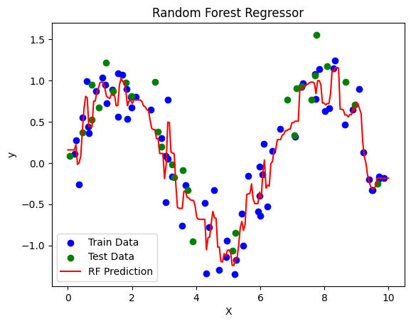
1. Dataset: \(y = \sin(X) + \text{noise}\) → nonlinear regression example.

2. Random Forest Regressor:

   • 100 trees (n_estimators=100)

   • Trains independently on bootstrapped samples

   • Uses random subset of features at each split (max_features='auto')

   • oob_score=True gives an unbiased performance estimate using Out-of-Bag samples.

3. Metrics:

   • Train R² → how well model fits training data

   • Test R² → generalization performance

   • RMSE → error magnitude

4. Visualization:

   • Red curve → Random Forest predictions

   • Blue/Green points → training/test data

5. Feature Importance:

   • Shows which features contributed most to reducing variance (useful if multiple features exist)

---

Key Takeaways

• Random Forest averages predictions of many trees, reducing variance.

• Handles nonlinear relationships naturally.

• Out-of-Bag evaluation provides built-in validation.

• Hyperparameters like max_depth, min_samples_leaf, and n_estimators are crucial to avoid overfitting or underfitting.