Logistic Regression#
Linear Regression Limitation#
Linear regression is not suitable for classification because:
Output Range:
Linear regression predicts continuous values (−∞ to +∞).
Classification needs bounded probabilities (0 to 1). Predictions outside [0,1] cannot be interpreted as valid class probabilities.
Decision Boundary:
If you force a threshold (e.g., ≥0.5 → class 1, else class 0), the model assumes a linear relationship between input features and probability of class. Real-world class separation is often nonlinear.
Violation of Assumptions:
Linear regression assumes homoscedasticity and normally distributed errors.
Classification problems involve heteroscedasticity (variance changes with class), violating these assumptions.
Multiple Classes:
Linear regression cannot naturally extend to multi-class classification. Logistic regression or SVM handle this better.
Sensitivity to Outliers:
Outliers can push regression predictions far outside the [0,1] range, distorting classification thresholds.
Because of these issues, logistic regression or classification-specific algorithms (e.g., SVM, decision trees) are preferred.
How Logsitic Regression solves the problem#
Logistic regression solves the problems of using linear regression for classification in these ways:
Bounded Outputs:
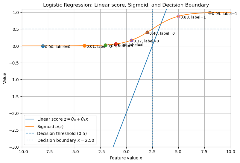
Logistic regression uses the sigmoid function:
\[ p(x) = \frac{1}{1 + e^{-(\beta_0 + \beta_1 x)}} \]This maps predictions to the range [0,1], making them interpretable as probabilities.
Decision Boundary:
The probability threshold (commonly 0.5) defines the decision boundary.
The boundary is still linear in the feature space, but probabilities are modeled correctly.
Error Distribution:
Logistic regression does not assume normality of errors.
Instead, it uses maximum likelihood estimation (MLE) to find parameters that best fit the classification problem.
Robustness to Outliers:
While not immune, logistic regression is less sensitive than linear regression because extreme predictions are squashed by the sigmoid.
Extension to Multiple Classes:
Logistic regression extends to multi-class problems through one-vs-rest (OvR) or multinomial logistic regression (softmax regression).
In short:
Linear regression → predicts unbounded values, unsuitable for probability.
Logistic regression → predicts bounded probabilities, explicitly designed for classification.
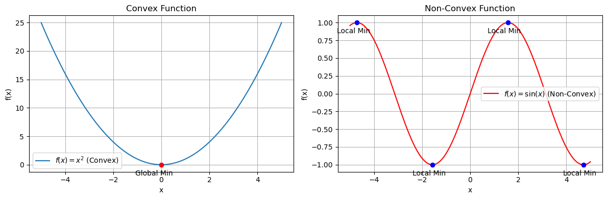
Convex and Non-Convex function#
A convex function has a bowl-shaped curve, while a non-convex function can have multiple dips and peaks.
Convex function#
Definition: A function \(f(x)\) is convex if for any two points \(x_1, x_2\) in its domain and any \(\lambda \in [0,1]\):
\[ f(\lambda x_1 + (1-\lambda)x_2) \leq \lambda f(x_1) + (1-\lambda)f(x_2) \]Visual property: The line segment between any two points on the curve lies above or on the curve.
Optimization:
Has a single global minimum.
Gradient Descent is guaranteed to converge.
Examples:
\(f(x) = x^2\)
Logistic Regression cost function (Log Loss).
Non-convex function#
Definition: Fails the convex inequality above.
Visual property: The curve has multiple local minima/maxima.
Optimization:
Gradient Descent can get stuck in a local minimum instead of the global one.
Requires advanced methods (random restarts, stochastic optimization).
Examples:
\(f(x) = \sin(x)\)
Mean Squared Error applied to Logistic Regression.
Deep Neural Network loss surfaces.
👉 In Logistic Regression, the log loss cost function is convex, ensuring a single minimum. In contrast, if we incorrectly used squared error, the cost would be non-convex, making training unstable.
import numpy as np
import matplotlib.pyplot as plt

# Define functions
x = np.linspace(-5, 5, 400)
convex_func = x**2
nonconvex_func = np.sin(x)

# Find minima for convex (single global min at x=0)
convex_min_x = 0
convex_min_y = convex_min_x**2

# For non-convex (local minima)
local_minima_x = [-3*np.pi/2, -np.pi/2, np.pi/2, 3*np.pi/2]  # approximate within range
local_minima_x = [val for val in local_minima_x if -5 <= val <= 5]
local_minima_y = [np.sin(val) for val in local_minima_x]

# Create side-by-side subplots
fig, axes = plt.subplots(1, 2, figsize=(12, 4))

# Convex function plot
axes[0].plot(x, convex_func, label=r"$f(x) = x^2$ (Convex)")
axes[0].scatter(convex_min_x, convex_min_y, color='red', zorder=5)
axes[0].annotate("Global Min", (convex_min_x, convex_min_y), textcoords="offset points", xytext=(-10,-15), ha='center')
axes[0].set_title("Convex Function")
axes[0].set_xlabel("x")
axes[0].set_ylabel("f(x)")
axes[0].legend()
axes[0].grid(True)

# Non-convex function plot
axes[1].plot(x, nonconvex_func, label=r"$f(x) = \sin(x)$ (Non-Convex)", color="red")
axes[1].scatter(local_minima_x, local_minima_y, color='blue', zorder=5)
for xi, yi in zip(local_minima_x, local_minima_y):
    axes[1].annotate("Local Min", (xi, yi), textcoords="offset points", xytext=(-5,-15), ha='center')
axes[1].set_title("Non-Convex Function")
axes[1].set_xlabel("x")
axes[1].set_ylabel("f(x)")
axes[1].legend()
axes[1].grid(True)

plt.tight_layout()
plt.show()
# Generating a single plot showing the linear score z, its sigmoid, and decision boundary.
import numpy as np
import matplotlib.pyplot as plt

# Parameters
theta0 = -2.0
theta1 = 0.8

# Input range
x = np.linspace(-10, 10, 400)
z = theta0 + theta1 * x
sigmoid = 1 / (1 + np.exp(-z))

# Sample points to illustrate classification
x_samples = np.array([-8, -4, -2, -1, 0.5, 2, 5, 8])
z_samples = theta0 + theta1 * x_samples
probs_samples = 1 / (1 + np.exp(-z_samples))
labels = (probs_samples >= 0.5).astype(int)

plt.figure(figsize=(9,6))
plt.plot(x, z, label='Linear score $z=\\theta_0+\\theta_1 x$')
plt.plot(x, sigmoid, label='Sigmoid $\\sigma(z)$')
plt.axhline(0.5, linestyle='--', label='Decision threshold (0.5)')
# Decision boundary where z = 0 -> x = -theta0/theta1
x_boundary = -theta0 / theta1
plt.axvline(x_boundary, linestyle=':', label=f'Decision boundary $x={x_boundary:.2f}$')

# Plot sample points and their probabilities
for xi, pi, li in zip(x_samples, probs_samples, labels):
    plt.scatter([xi], [pi], s=60)
    plt.text(xi + 0.2, pi - 0.06, f'{pi:.2f}, label={li}', fontsize=9)

plt.xlabel('Feature value $x$')
plt.ylabel('Value')
plt.title('Logistic Regression: Linear score, Sigmoid, and Decision Boundary')
plt.legend()
plt.grid(True)
plt.ylim(-3, 1.1)
plt.xlim(x.min(), x.max())
plt.show()
Why Linear Regression Fails for Classification#
Outliers: The best-fit line can be heavily influenced by extreme values.
Output Range: Linear regression can produce outputs less than 0 or greater than 1, which are invalid for probabilities.
Solution: Logistic Regression#
Apply a squashing function to the linear output to constrain predictions between 0 and 1.
The sigmoid (logistic) function is used:
Key properties:
Outputs always between 0 and 1.
Midpoint at 0.5 when \(z = 0\).
If \(z > 0\), \(\sigma(z) > 0.5\).
Hypothesis function with sigmoid:
For multiple features:
Cost Function#
Linear regression cost function leads to non-convexity when combined with sigmoid, causing local minima.
Logistic regression uses log loss (cross-entropy) for convexity:
Combined form:
Ensures convexity, allowing gradient descent to reliably find the global minimum.
Gradient Descent#
Parameter update rule:
Repeat until convergence.
For multiple features, update each \(\theta_j\) in the same way.
Summary#
Fit a linear model: \(\theta_0 + \theta_1 x_1 + \dots\)
Apply sigmoid activation to squash outputs between 0 and 1.
Use log loss to ensure a convex cost function.
Optimize parameters using gradient descent.
Predictions can now be interpreted as probabilities for classification.