Cost Function#
Reminder: What SVR Does#
SVR doesn’t try to predict exactly each data point.
Instead, it tries to find a function \(f(x) = w^T \phi(x) + b\) that keeps predictions within a tolerance zone (ε-tube) around the actual values.
Errors inside the ε-tube are ignored.
Errors outside the ε-tube are penalized.
SVR Cost Function#
The optimization problem is:
Subject to:
Explanation of Each Term#
\(\frac{1}{2}\|w\|^2\) → margin maximization (we want the flattest function).
\(C \sum (\xi_i + \xi_i^*)\) → penalty for deviations outside ε.
\(\epsilon\) → size of the tolerance tube.
\(\xi_i, \xi_i^*\) → slack variables, measure how far outside the tube a point lies.
ε-insensitive Loss Function#
The SVR loss is also called the ε-insensitive loss:
👉 Interpretation:
If prediction is within ±ε of actual → no cost.
If prediction lies outside → cost grows linearly with distance from the ε-boundary.
Role of Hyperparameters in Cost#
C (Regularization parameter):
High C → penalizes errors more strongly → tighter fit → may overfit.
Low C → allows more slack → smoother function.
ε (Epsilon-insensitive zone):
Larger ε → fewer support vectors, simpler model.
Smaller ε → more support vectors, sensitive fit.
γ (Kernel parameter, e.g. in RBF):
Controls influence of each training point.
High γ → each point has small radius of influence → wiggly fit.
Low γ → smoother fit.
Visualization of ε-tube Intuition#
Imagine the regression line with a tube around it:
Points inside the tube → cost = 0.
Points outside → cost = distance beyond tube.
This is what makes SVR robust — it ignores small deviations and only cares about big errors.
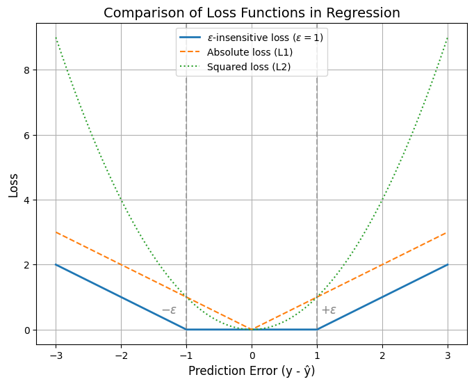
Comparison with Other Losses#
Linear Regression (OLS): Uses squared loss \((y - \hat{y})^2\).
Lasso Regression: Uses absolute loss \(|y - \hat{y}|\).
SVR: Uses ε-insensitive loss, which blends the two ideas by ignoring small errors and penalizing big ones linearly.
Summary: The SVR cost function balances two goals:
Keep the regression function as flat as possible (\(\frac{1}{2}\|w\|^2\)).
Minimize large prediction errors (ε-insensitive loss, controlled by \(C\)).
import numpy as np
import matplotlib.pyplot as plt

# Define loss functions
def epsilon_insensitive_loss(y_true, y_pred, epsilon=1.0):
    error = np.abs(y_true - y_pred)
    return np.maximum(0, error - epsilon)

def squared_loss(y_true, y_pred):
    return (y_true - y_pred) ** 2

def absolute_loss(y_true, y_pred):
    return np.abs(y_true - y_pred)

# Range of prediction errors
errors = np.linspace(-3, 3, 400)
y_true = 0  # assume true value = 0
y_pred = errors  # predictions offset from 0

# Loss values
eps_loss = epsilon_insensitive_loss(y_true, y_pred, epsilon=1.0)
sq_loss = squared_loss(y_true, y_pred)
abs_loss = absolute_loss(y_true, y_pred)

# Plot
plt.figure(figsize=(8,6))
plt.plot(errors, eps_loss, label=r'$\epsilon$-insensitive loss ($\epsilon=1$)', linewidth=2)
plt.plot(errors, abs_loss, label='Absolute loss (L1)', linestyle='--')
plt.plot(errors, sq_loss, label='Squared loss (L2)', linestyle=':')

# Add vertical lines for epsilon boundaries
plt.axvline(x=1, color='gray', linestyle='--', alpha=0.6)
plt.axvline(x=-1, color='gray', linestyle='--', alpha=0.6)
plt.text(1.05, 0.5, r'$+\epsilon$', fontsize=12, color='gray')
plt.text(-1.4, 0.5, r'$-\epsilon$', fontsize=12, color='gray')

plt.title("Comparison of Loss Functions in Regression", fontsize=14)
plt.xlabel("Prediction Error (y - ŷ)", fontsize=12)
plt.ylabel("Loss", fontsize=12)
plt.legend()
plt.grid(True)
plt.show()