Bias, Variance, and Their Trade-off

Bias, Variance, and Their Trade-off #

Bias #

Bias measures how far a model’s predictions are from the true underlying function.

Mathematically, for estimator \(\hat{f}(x)\):

\[ \text{Bias}(x) = \mathbb{E}[\hat{f}(x)] - f(x) \]

Interpretation:

High bias = model is too simple.
Leads to underfitting.
Model learns only coarse patterns and ignores important structure.

Examples:

Using linear regression for a non-linear problem.
Using few decision tree splits.

Effects:

High training error
High testing error
Model predictions look overly smooth or simplistic.

Variance #

Variance measures how sensitive the model is to small fluctuations in training data.

\[ \text{Variance}(x) = \mathbb{E}\big[(\hat{f}(x) - \mathbb{E}[\hat{f}(x)])^2\big] \]

Interpretation:

High variance = model is too complex.
Leads to overfitting.
The model memorizes noise instead of learning general patterns.

Examples:

Deep decision trees
High-degree polynomial regression
kNN with very small (k)

Effects:

Low training error
High testing error
Model curves wildly to chase noise in data.

Total Error (Bias–Variance Decomposition)**#

For a regression problem with:

True function \(f(x)\),
Model prediction \(\hat{f}(x)\),
Noise variance \(\sigma^2\),

Expected prediction error at point (x) is:

\[ \begin{align}\begin{aligned} \mathbb{E}[(y - \hat{f}(x))^2] = \underbrace{\text{Bias}^2}_{\text{error from wrong assumptions}}\\* \underbrace{\text{Variance}}_{\text{error from sensitivity}} * \underbrace{\sigma^2}_{\text{irreducible noise}} \end{aligned}\end{align} \]

Irreducible noise cannot be removed.

The Bias–Variance Trade-off #

A model cannot simultaneously minimize both bias and variance; improving one often worsens the other.

Model Complexity	Bias	Variance	Behavior
Low	High	Low	Underfitting
Medium	Medium	Medium	Optimal zone
High	Low	High	Overfitting

Key insight:

Increasing model complexity decreases bias but increases variance.
Decreasing complexity increases bias but decreases variance.

Goal: Choose complexity that balances both → lowest test error.

How to Reduce Bias #

Use when model is too simple.

Add more features
Use more complex models
Reduce regularization ((\lambda))
Increase model capacity (depth, degree, layers)

How to Reduce Variance #

Use when the model is too sensitive.

Add regularization (L1, L2)
Reduce model complexity
Use dropout (for NN)
Use fewer polynomial degrees
Prune trees or limit tree depth
Increase training data
Use bagging / random forests

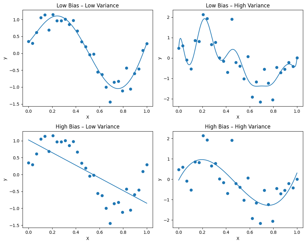
Visualization Summary #

High Bias: Predicts wrong shape; consistently incorrect.
High Variance: Predicts wildly different shapes for small data changes.
Balanced: Captures structure without fitting noise.

import numpy as np
import matplotlib.pyplot as plt
from math import ceil, sqrt

# Example: models dict
# models = { "Low Bias – Low Variance": model1, ... }

n = len(models)                        # number of plots
cols = ceil(sqrt(n))                   # square-like arrangement
rows = ceil(n / cols)

plt.figure(figsize=(cols * 5, rows * 4))

for i, (title, model) in enumerate(models.items(), 1):
    if "High Variance" in title:
        y_used = y + noise_extra
    else:
        y_used = y

    model.fit(X, y_used)
    X_test = np.linspace(0, 1, 200).reshape(-1, 1)
    y_pred = model.predict(X_test)

    ax = plt.subplot(rows, cols, i)
    ax.scatter(X, y_used)
    ax.plot(X_test, y_pred)
    ax.set_title(title)
    ax.set_xlabel("X")
    ax.set_ylabel("y")

plt.tight_layout()
plt.show()

../../_images/49861ab2dd0251219226dbfa1b4d3004242fdd7cc9cc77019d196be2754022a4.png

Bias, Variance, and Their Trade-off

Contents