Bias–Variance Tradeoff#
The Bias–Variance Tradeoff is a core concept in machine learning that explains the balance between underfitting and overfitting.
Bias#
Definition: Error caused by simplifying a model too much and ignoring real patterns in the data.
High Bias → Model is too simple → Underfitting.
Example: Using a straight line to fit a highly curved pattern.
Effect: Predictions are consistently wrong in the same direction.
Variance#
Definition: Error caused by making a model too complex and fitting even the noise in the training data.
High Variance → Model is too sensitive to small changes in the data → Overfitting.
Example: A polynomial of degree 15 fitting just 10 data points.
Effect: Model performs well on training data but poorly on unseen data.
The Tradeoff#
Increasing model complexity → Bias decreases, Variance increases.
Decreasing model complexity → Bias increases, Variance decreases.
Goal: Find the “sweet spot” where both bias and variance are low enough to minimize total error.
Error Decomposition#
The total error in a model can be expressed as:
Bias²: Squared error from wrong assumptions.
Variance: Error from sensitivity to training data.
Irreducible Error: Noise in the data we can’t remove.
Visual Representation#
Imagine a dartboard 🎯:
High Bias, Low Variance: All darts land far from the bullseye, but close to each other (consistently wrong).
Low Bias, High Variance: Darts scatter all over the board (inconsistent).
High Bias, High Variance: Darts are scattered and far from the bullseye.
Low Bias, Low Variance: Darts cluster around the bullseye (ideal model).
Formula for Bias–Variance Tradeoff#
The expected squared error at a point \(x\) is:
Where:
\(\hat{f}(x)\) = predicted value from the model.
\(y\) = true value.
\(\sigma^2\) = variance of noise in the data.
import numpy as np
import matplotlib.pyplot as plt
from sklearn.preprocessing import PolynomialFeatures
from sklearn.linear_model import LinearRegression
from sklearn.metrics import mean_squared_error
from sklearn.model_selection import train_test_split

# Generate synthetic data
np.random.seed(42)
X = np.sort(np.random.rand(50) * 6 - 3)[:, np.newaxis]  # -3 to 3 range
y = np.sin(X) + np.random.normal(0, 0.2, X.shape)  # sin curve + noise

# Train-test split
X_train, X_test, y_train, y_test = train_test_split(X, y, test_size=0.3, random_state=42)

degrees = [1, 4, 15]  # Low, medium, high complexity
plt.figure(figsize=(15, 8))

for i, degree in enumerate(degrees, 1):
    # Polynomial features
    poly = PolynomialFeatures(degree=degree)
    X_train_poly = poly.fit_transform(X_train)
    X_test_poly = poly.transform(X_test)

    # Fit model
    model = LinearRegression()
    model.fit(X_train_poly, y_train)

    # Predictions
    y_pred_train = model.predict(X_train_poly)
    y_pred_test = model.predict(X_test_poly)

    # Error calculation (as proxy for bias & variance)
    train_error = mean_squared_error(y_train, y_pred_train)
    test_error = mean_squared_error(y_test, y_pred_test)

    # Plot
    plt.subplot(1, 3, i)
    X_range = np.linspace(-3, 3, 100).reshape(-1, 1)
    X_range_poly = poly.transform(X_range)
    y_range_pred = model.predict(X_range_poly)

    plt.scatter(X_train, y_train, color="blue", alpha=0.5, label="Train Data")
    plt.scatter(X_test, y_test, color="green", alpha=0.5, label="Test Data")
    plt.plot(X_range, y_range_pred, color="red", label="Model Prediction")
    plt.title(f"Degree {degree}\nTrain Err: {train_error:.3f}, Test Err: {test_error:.3f}")
    plt.legend()

plt.suptitle("Bias-Variance Tradeoff: Underfitting → Good Fit → Overfitting", fontsize=16)
plt.show()
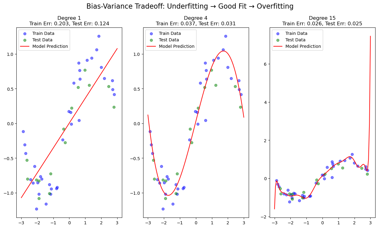
How to Read the Results#
Degree 1 → High Bias: The line is too simple to capture the sine curve → Underfits → Both train & test errors high.
Degree 4 → Low Bias, Low Variance: Fits well without overfitting → Sweet spot → Errors are low.
Degree 15 → Low Bias but High Variance: Fits noise in training data → Train error low, test error high → Overfits.