Cost Function#
The goal of K-Means is to partition the dataset into \(K\) clusters such that points within each cluster are as similar as possible (intra-cluster similarity is high) and as dissimilar as possible from other clusters (inter-cluster separation is high).
To formalize this, K-Means uses a cost function called the Sum of Squared Errors (SSE) or Within-Cluster Sum of Squares (WCSS).
1. Within-Cluster Sum of Squares (WCSS / Inertia)#
The main cost function is:
where:
\(K\) = number of clusters
\(C_k\) = set of points assigned to cluster \(k\)
\(x_i\) = data point
\(\mu_k\) = centroid of cluster \(k\)
\(\| x_i - \mu_k \|^2\) = squared Euclidean distance between point and cluster centroid
👉 This means K-Means tries to minimize the squared distance of each point to its cluster center.
2. Between-Cluster Separation (Optional, Not Explicit in Vanilla K-Means)#
Though not explicitly optimized by K-Means, ideally clusters should also be well-separated. A related measure is the Between-Cluster Sum of Squares (BCSS):
where:
\(n_k\) = number of points in cluster \(k\)
\(\mu\) = global mean of all points
👉 A good clustering should have low WCSS (compact clusters) and high BCSS (well-separated clusters).
3. Objective in Optimization#
Vanilla K-Means → minimizes WCSS only.
Implicitly → this indirectly improves BCSS, because minimizing intra-cluster variance generally increases inter-cluster separation.
Intuition Behind the Cost Function#
If all points are very close to their centroids → \(J\) is small → good clustering.
If points are scattered far from centroids → \(J\) is large → poor clustering.
K-Means works by iteratively reassigning points and updating centroids to reduce \(J\) at every step until convergence.
So the main cost function in K-Means is:
Sum of Squared Distances of points to their nearest centroid (WCSS).
import numpy as np
import matplotlib.pyplot as plt
from sklearn.datasets import make_blobs
from sklearn.cluster import KMeans
# 1. Generate synthetic dataset
X, y = make_blobs(n_samples=300, centers=4, cluster_std=0.7, random_state=42)
# 2. Run KMeans with different iterations to track cost (WCSS)
kmeans = KMeans(n_clusters=4, init="random", n_init=1, max_iter=1, random_state=42)
# Store inertia (WCSS) per iteration
costs = []
# Run manually for multiple iterations
for i in range(1, 11): # 10 iterations
kmeans.max_iter = i
kmeans.fit(X)
costs.append(kmeans.inertia_) # inertia_ = WCSS
# 3. Final clustering with 4 clusters for visualization
final_kmeans = KMeans(n_clusters=4, random_state=42)
final_kmeans.fit(X)
y_pred = final_kmeans.predict(X)
# 4. Plot
plt.figure(figsize=(12,5))
# Plot cost function over iterations
plt.subplot(1,2,1)
plt.plot(range(1,11), costs, marker="o", color="blue")
plt.xlabel("Iterations")
plt.ylabel("WCSS (Inertia)")
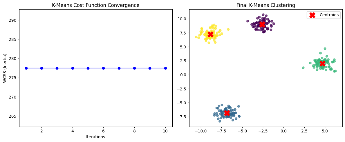
plt.title("K-Means Cost Function Convergence")
# Plot final clustered data
plt.subplot(1,2,2)
plt.scatter(X[:,0], X[:,1], c=y_pred, cmap="viridis", s=30, alpha=0.7)
plt.scatter(final_kmeans.cluster_centers_[:,0], final_kmeans.cluster_centers_[:,1],
c="red", s=200, marker="X", label="Centroids")
plt.title("Final K-Means Clustering")
plt.legend()
plt.tight_layout()
plt.show()