KNN Variants#
One limitation of standard K-Nearest Neighbors (KNN) is that finding the nearest neighbors requires computing the distance to all points in the dataset.
If there are \(n\) points, this is O(n) time complexity per query, which is inefficient for large datasets.
To optimize this, we use spatial data structures like K-d Tree and Ball Tree.
1. K-d Tree (k-dimensional Tree)#
Idea#
A binary tree that partitions the data space along feature axes (dimensions).
At each node, the data is split based on the median value of a particular dimension, alternating between dimensions at each level.
This creates hierarchical regions, so you don’t need to check all points during a search.
Construction#
Start with all points.
Select a dimension (e.g., x-axis = feature F1 for the first split).
Compute the median of that dimension.
Split the points into two groups:
Left subtree: points ≤ median
Right subtree: points > median
Alternate dimensions at each level (e.g., F1 → F2 → F1 → …)
Recursively split each region until each leaf node has a small number of points.
Example#
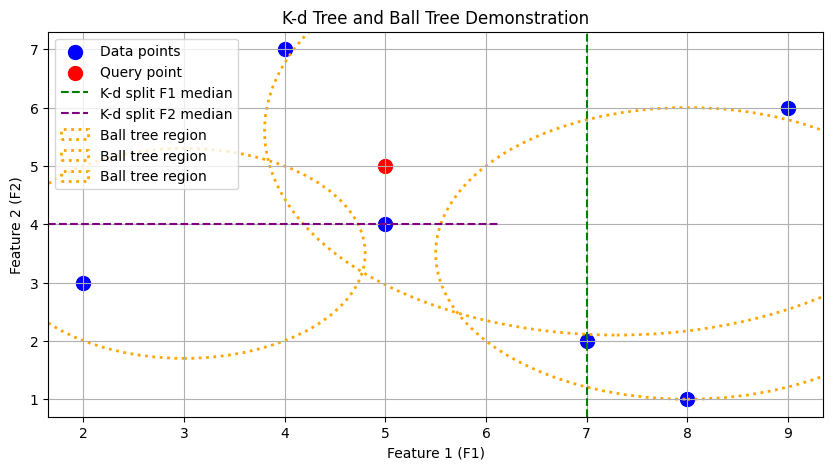
Suppose points: (7,2), (5,4), (4,7), (2,3), (8,1), (9,6)
First split: median F1 = 7 → splits points into left (≤7) and right (>7)
Second split: median F2 of left points = 4 → splits left region into top and bottom
Repeat recursively, alternating F1 and F2.
Searching#
To find the nearest neighbors:
Traverse the tree to locate the region containing the query point.
Compute distances only within this region first.
Backtracking is used to check neighboring regions if necessary for additional nearest neighbors.
This drastically reduces the number of distance computations compared to brute-force search.
2. Ball Tree#
Idea#
A Ball Tree groups points based on proximity, enclosing them in hyperspheres (balls).
Unlike K-d Tree, Ball Tree uses distance-based grouping, not axis-aligned splits.
Construction#
Start with all points.
Cluster nearby points together into groups.
Each group forms a “ball” with a center and radius covering all its points.
Recursively combine balls into larger parent balls until all points are included in a root ball.
Example#
Suppose points: 1,2,3,4,5,6,7,8,9
Step 1: Create small groups:
G1 = {1,2}, G2 = {3,4}, G3 = {5,6,7}, G4 = {8,9}
Step 2: Merge nearby groups:
G5 = merge(G1,G2), G6 = merge(G3,G4)
Step 3: Merge top-level groups:
G7 = merge(G5,G6) → root
Each ball represents a spatial region for efficient neighbor search.
Searching#
For a new query point:
Start at the root ball.
Check if the query lies within a ball → only compute distances within relevant balls.
Traverse down the hierarchy to find nearest points.
No backtracking is usually needed if the query is far from other balls, making it faster than K-d Tree in some cases.
3. Benefits of K-d Tree and Ball Tree#
Feature |
K-d Tree |
Ball Tree |
|---|---|---|
Splitting |
Axis-aligned, alternating |
Distance-based (spherical) |
Backtracking |
Required for accurate nearest neighbors |
Often minimized |
Best for |
Low-dimensional data |
High-dimensional data |
Complexity |
O(log n) per search (average) |
O(log n) per search (average) |
Both trees reduce time complexity from O(n) to roughly O(log n) per query.
Instead of computing distances to all points, we prune large portions of the dataset that cannot contain the nearest neighbors.
4. Intuition Summary#
K-d Tree
Imagine slicing the space along x and y axes repeatedly.
Query points only need to check the slice they belong to and nearby slices.
Ball Tree
Imagine enclosing points in balls.
Query points only search balls near them, skipping faraway groups entirely.
Overall Goal: Reduce distance computations → faster KNN search → scalable for larger datasets.
import matplotlib.pyplot as plt
from sklearn.neighbors import KDTree, BallTree
import numpy as np

# Sample 2D data points
X = np.array([[7,2], [5,4], [4,7], [2,3], [8,1], [9,6]])

# Query point
query = np.array([[5,5]])

# Plot original points and query
plt.figure(figsize=(10,5))

plt.scatter(X[:,0], X[:,1], c='blue', label='Data points', s=100)
plt.scatter(query[:,0], query[:,1], c='red', label='Query point', s=100)

# Plot K-d tree splits (manually for demonstration, approximate)
plt.axvline(x=7, color='green', linestyle='--', label='K-d split F1 median')
plt.axhline(y=4, xmin=0.0, xmax=0.58, color='purple', linestyle='--', label='K-d split F2 median')

# Plot Ball Tree circles (center + radius covering points in a ball)
ball_centers = np.array([[3,3.5],[8,3.5],[7.3,5.6]])
ball_radii = [1.8, 2.5, 3.5]

for center, r in zip(ball_centers, ball_radii):
    circle = plt.Circle(center, r, color='orange', fill=False, linestyle=':', linewidth=2, label='Ball tree region')
    plt.gca().add_patch(circle)

plt.xlabel('Feature 1 (F1)')
plt.ylabel('Feature 2 (F2)')
plt.title('K-d Tree and Ball Tree Demonstration')
plt.legend(loc='upper left')
plt.grid(True)
plt.show()