XGBoost Classifier#
XGBoost Classifier is a gradient boosting-based algorithm optimized for classification tasks (binary or multiclass). It is widely used because it is fast, accurate, and regularized.
1. Intuition#
Think of XGBoost as a team of weak learners (decision trees) that work together to fix each other’s mistakes:
Start with a simple prediction (e.g., log-odds of positive class).
Fit a decision tree to the residual errors or gradients of loss function.
Update predictions by adding the new tree with a learning rate (shrinkage).
Repeat for many rounds until convergence or stopping criteria.
➡️ The model improves sequentially, focusing more on hard-to-classify samples.
2. Workflow of XGBClassifier#
Input data → Features (X), labels (y).
Initialize predictions (log-odds of classes).
Compute gradients & hessians (1st and 2nd derivatives of the loss).
Build a decision tree:
Use gradients & hessians to decide splits.
Find the best split by maximizing gain (improvement in loss).
Update predictions with the tree’s output, scaled by
learning_rate.Repeat steps 3–5 until
n_estimatorsis reached or early stopping triggers.Final prediction: apply softmax/logistic function to convert scores → probabilities → class labels.
3. Objective Functions in Classification#
XGBoost supports multiple loss functions:
Binary Classification Logistic loss:
\[ L = -\sum_{i=1}^n \big[ y_i \log(p_i) + (1-y_i) \log(1-p_i) \big] \]where \(p_i = \sigma(\hat{y}_i)\), sigmoid converts score → probability.
Multiclass Classification Softmax loss:
\[ L = -\sum_{i=1}^n \sum_{k=1}^K y_{ik} \log(p_{ik}) \]where \(p_{ik} = \frac{e^{\hat{y}_{ik}}}{\sum_j e^{\hat{y}_{ij}}}\).
4. Important Hyperparameters#
n_estimators→ number of boosting rounds.learning_rate→ step size shrinkage (avoids overfitting).max_depth→ depth of trees (controls complexity).subsample→ fraction of training samples per tree.colsample_bytree→ fraction of features per tree.reg_lambda,reg_alpha→ L2/L1 regularization.objective→"binary:logistic","multi:softmax","multi:softprob".
5. Evaluation Metrics#
Binary: Accuracy, Precision, Recall, F1, AUC-ROC.
Multiclass: Accuracy, Log-loss, Macro/Micro F1.
6. Advantages of XGBClassifier#
Very fast and efficient (parallel & GPU support).
Handles missing values automatically.
Supports regularization (avoids overfitting).
Can handle imbalanced datasets via
scale_pos_weight.Works with large datasets and high dimensions.
7. When to Use XGBClassifier#
Binary classification (spam vs not spam, fraud detection).
Multiclass classification (digit recognition, disease type prediction).
Tabular datasets where boosting trees outperform deep learning.
# ------------------------------
# XGBClassifier Demonstration (Fixed)
# ------------------------------
import numpy as np
import matplotlib.pyplot as plt
from sklearn.datasets import make_classification
from sklearn.model_selection import train_test_split
from sklearn.metrics import accuracy_score, classification_report, ConfusionMatrixDisplay
from xgboost import XGBClassifier, plot_importance
import warnings
warnings.filterwarnings("ignore")
# 1. Generate synthetic classification dataset
X, y = make_classification(
n_samples=500, n_features=10, n_informative=6, n_redundant=2,
n_classes=2, random_state=42
)
# Split into train/test
X_train, X_test, y_train, y_test = train_test_split(
X, y, test_size=0.2, random_state=42
)
# 2. Train XGBClassifier
model = XGBClassifier(
n_estimators=200, # number of boosting rounds
learning_rate=0.1, # shrinkage
max_depth=3, # depth of trees
subsample=0.8, # row sampling
colsample_bytree=0.8, # feature sampling
reg_lambda=1, # L2 regularization
use_label_encoder=False, # suppress deprecation warning
eval_metric="logloss", # specify metric to avoid warnings
random_state=42
)
model.fit(X_train, y_train)
# 3. Predictions
y_pred = model.predict(X_test)
# 4. Evaluate performance
print("✅ Accuracy:", accuracy_score(y_test, y_pred))
print("\nClassification Report:\n", classification_report(y_test, y_pred))
# 5. Feature importance and confusion matrix
fig, axes = plt.subplots(1, 2, figsize=(10, 6))
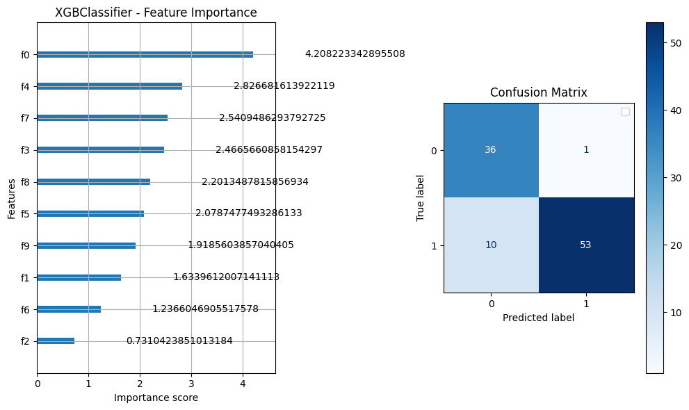
# Feature importance
plot_importance(model, importance_type="gain", ax=axes[0])
axes[0].set_title("XGBClassifier - Feature Importance")
# Confusion matrix
ConfusionMatrixDisplay.from_estimator(model, X_test, y_test, cmap="Blues", ax=axes[1])
axes[1].set_title("Confusion Matrix")
plt.legend()
plt.tight_layout()
plt.show()
✅ Accuracy: 0.89

Classification Report:
               precision    recall  f1-score   support

           0       0.78      0.97      0.87        37
           1       0.98      0.84      0.91        63

    accuracy                           0.89       100
   macro avg       0.88      0.91      0.89       100
weighted avg       0.91      0.89      0.89       100