Performance Metrics#
1. Internal Metrics (without ground truth)#
These measure the quality of clusters based on compactness and separation.
(a) Inertia (Within-Cluster Sum of Squares, WCSS)#
Definition: The sum of squared distances between each point and its assigned cluster centroid.
Formula:
\[ WCSS = \sum_{k=1}^{K} \sum_{x_i \in C_k} \| x_i - \mu_k \|^2 \]where \(C_k\) is cluster \(k\), and \(\mu_k\) its centroid.
Goal: Minimize inertia (lower is better).
Limitation: Always decreases as \(K\) increases (can overfit).
(b) Silhouette Score#
Definition: Measures how similar a point is to its own cluster vs. other clusters.
Formula: For a point \(i\):
\[ s(i) = \frac{b(i) - a(i)}{\max(a(i), b(i))} \]where:
\(a(i)\): average distance from \(i\) to points in the same cluster.
\(b(i)\): average distance from \(i\) to points in the nearest other cluster.
Range: -1 to 1
\(\approx 1\): well-clustered
\(\approx 0\): overlapping clusters
\(< 0\): misclassified
Goal: Higher silhouette score is better.
(c) Davies–Bouldin Index (DBI)#
Definition: Measures the average similarity between clusters (compactness + separation).
Formula:
\[ DBI = \frac{1}{K} \sum_{i=1}^{K} \max_{j \ne i} \frac{\sigma_i + \sigma_j}{d(\mu_i, \mu_j)} \]where:
\(\sigma_i\): average distance of points in cluster \(i\) to centroid \(\mu_i\).
\(d(\mu_i, \mu_j)\): distance between centroids of clusters \(i\) and \(j\).
Goal: Minimize DBI (lower is better).
(d) Calinski–Harabasz Index (Variance Ratio Criterion)#
Definition: Ratio of between-cluster dispersion to within-cluster dispersion.
Formula:
\[ CH = \frac{Tr(B_k)}{Tr(W_k)} \cdot \frac{N-K}{K-1} \]where:
\(B_k\): between-cluster dispersion matrix.
\(W_k\): within-cluster dispersion matrix.
\(N\): number of samples.
\(K\): number of clusters.
Goal: Higher is better (more separated and compact clusters).
2. External Metrics (when ground truth labels exist)#
These compare clustering results with true labels.
(a) Adjusted Rand Index (ARI)#
Measures similarity between predicted clusters and true labels, corrected for chance.
Range: -1 to 1 (1 = perfect match, 0 = random, -1 = bad clustering).
(b) Normalized Mutual Information (NMI)#
Measures shared information between clusters and true labels.
Range: 0 to 1 (1 = perfect match).
(c) Homogeneity, Completeness, V-measure#
Homogeneity: Each cluster contains only members of one class.
Completeness: All members of a class are in the same cluster.
V-measure: Harmonic mean of homogeneity & completeness.
Summary Table
Metric |
Type |
Range |
Goal |
|---|---|---|---|
Inertia (WCSS) |
Internal |
≥ 0 |
Lower |
Silhouette Score |
Internal |
-1 to 1 |
Higher |
Davies–Bouldin Index |
Internal |
≥ 0 |
Lower |
Calinski–Harabasz |
Internal |
≥ 0 |
Higher |
Adjusted Rand Index |
External |
-1 to 1 |
Higher |
Normalized Mutual Information |
External |
0 to 1 |
Higher |
V-measure |
External |
0 to 1 |
Higher |
import numpy as np
import matplotlib.pyplot as plt
from sklearn.datasets import make_blobs
from sklearn.cluster import KMeans
from sklearn.metrics import (
silhouette_score, davies_bouldin_score, calinski_harabasz_score,
adjusted_rand_score, normalized_mutual_info_score, v_measure_score
)
# 1. Generate synthetic dataset with ground truth labels
X, y_true = make_blobs(n_samples=300, centers=3, cluster_std=0.7, random_state=42)
# 2. Apply KMeans clustering
kmeans = KMeans(n_clusters=3, random_state=42, n_init=10)
y_kmeans = kmeans.fit_predict(X)
# 3. Internal Metrics
inertia = kmeans.inertia_
silhouette = silhouette_score(X, y_kmeans)
dbi = davies_bouldin_score(X, y_kmeans)
ch = calinski_harabasz_score(X, y_kmeans)
# 4. External Metrics (since ground truth is known)
ari = adjusted_rand_score(y_true, y_kmeans)
nmi = normalized_mutual_info_score(y_true, y_kmeans)
v_measure = v_measure_score(y_true, y_kmeans)
# 5. Display Results
results = {
"Inertia (WCSS)": inertia,
"Silhouette Score": silhouette,
"Davies–Bouldin Index": dbi,
"Calinski–Harabasz Index": ch,
"Adjusted Rand Index": ari,
"Normalized Mutual Information": nmi,
"V-measure": v_measure
}
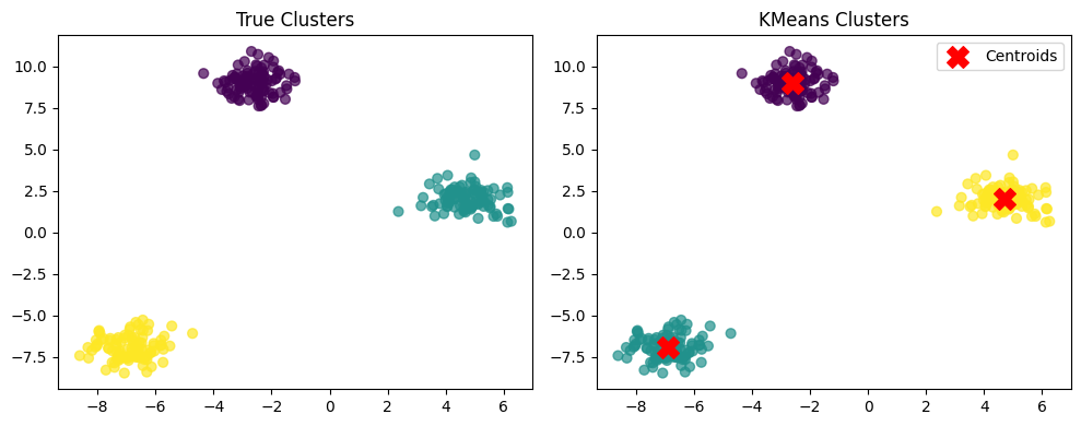
# 6. Plot clustering result
plt.figure(figsize=(10,4))
# True clusters
plt.subplot(1,2,1)
plt.scatter(X[:,0], X[:,1], c=y_true, cmap='viridis', s=40, alpha=0.7)
plt.title("True Clusters")
# KMeans predicted clusters
plt.subplot(1,2,2)
plt.scatter(X[:,0], X[:,1], c=y_kmeans, cmap='viridis', s=40, alpha=0.7)
plt.scatter(kmeans.cluster_centers_[:,0], kmeans.cluster_centers_[:,1], c='red', marker='X', s=200, label="Centroids")
plt.title("KMeans Clusters")
plt.legend()
plt.tight_layout()
plt.show()
results
{'Inertia (WCSS)': 277.76118005096237,
 'Silhouette Score': 0.8932417420300518,
 'Davies–Bouldin Index': 0.14928348889690027,
 'Calinski–Harabasz Index': 10542.407259542682,
 'Adjusted Rand Index': 1.0,
 'Normalized Mutual Information': 1.0,
 'V-measure': 1.0}