Cost Function#
DBSCAN does not use a cost function in the way algorithms like K-Means or PCA do. Instead, it is rule-based: clusters are defined by density conditions. Still, we can frame its logic mathematically.
1. Implicit Objective of DBSCAN#
The algorithm seeks a partition of dataset \(D\) into:
Clusters = maximal sets of density-connected points.
Noise = points not assigned to any cluster.
No optimization of a global scalar function happens. Instead, clustering emerges from local density checks.
2. Local Rules (instead of cost function)#
Neighborhood condition:
Core condition:
Cluster condition: Clusters are unions of points that are mutually density-connected.
3. Why no global cost function?#
DBSCAN does not optimize inter-cluster variance or distances.
It is deterministic given \(\epsilon\) and minPts.
Different parameter choices produce different clusterings.
4. How to evaluate DBSCAN output (proxy cost functions)#
Since there’s no internal objective, external metrics are used:
Silhouette coefficient
where \(a(i)\) = average intra-cluster distance, \(b(i)\) = nearest-cluster distance.
Davies–Bouldin Index: ratio of within-cluster scatter to between-cluster separation.
Adjusted Rand Index (ARI) or Mutual Information if ground-truth labels exist.
Summary
DBSCAN has no explicit cost function.
It uses density-based rules instead of optimization.
Quality of clustering is judged via external evaluation metrics.
import numpy as np
import matplotlib.pyplot as plt
from sklearn.datasets import make_moons, make_blobs
from sklearn.cluster import DBSCAN
from sklearn.metrics import silhouette_score, davies_bouldin_score, adjusted_rand_score

# Prepare datasets
X_moons, y_moons = make_moons(n_samples=300, noise=0.06, random_state=42)
X_blobs, y_blobs = make_blobs(n_samples=300, centers=[(-3, -3), (0, 0), (3, 3)],
                              cluster_std=[0.3, 1.0, 2.0], random_state=42)

datasets = [
    ("Moons (good for DBSCAN)", X_moons, y_moons, 0.25, 5),
    ("Blobs (varying density)", X_blobs, y_blobs, 0.6, 5),
]

results = []

for name, X, y_true, eps, minPts in datasets:
    db = DBSCAN(eps=eps, min_samples=minPts).fit(X)
    labels = db.labels_
    n_clusters = len(set(labels)) - (1 if -1 in labels else 0)
    n_noise = list(labels).count(-1)

    # Compute evaluation metrics when applicable
    metrics = {}
    metrics['n_clusters'] = n_clusters
    metrics['n_noise'] = n_noise
    metrics['eps'] = eps
    metrics['minPts'] = minPts

    if n_clusters >= 2:
        metrics['silhouette'] = silhouette_score(X, labels)
        metrics['davies_bouldin'] = davies_bouldin_score(X, labels)
    else:
        metrics['silhouette'] = None
        metrics['davies_bouldin'] = None

    # ARI vs ground truth (tolerates noise label -1)
    metrics['ARI'] = adjusted_rand_score(y_true, labels)

    results.append((name, X, labels, metrics))

# Print results
for name, X, labels, metrics in results:
    print(f"Dataset: {name}")
    print(f" eps={metrics['eps']}, minPts={metrics['minPts']}")
    print(f" Number of clusters (excluding noise): {metrics['n_clusters']}")
    print(f" Number of noise points: {metrics['n_noise']}")
    if metrics['silhouette'] is not None:
        print(f" Silhouette score: {metrics['silhouette']:.4f}")
        print(f" Davies-Bouldin index: {metrics['davies_bouldin']:.4f}")
    else:
        print(" Silhouette score: Not computed (requires >= 2 clusters)")
        print(" Davies-Bouldin index: Not computed (requires >= 2 clusters)")
    print(f" Adjusted Rand Index (vs true labels): {metrics['ARI']:.4f}")
    print("-" * 60)

# Plot each dataset separately as required
# Redo visualization with subplots for clarity
fig, axs = plt.subplots(1, 2, figsize=(12, 5))

for ax, (name, X, labels, metrics) in zip(axs, results):
    ax.scatter(X[:, 0], X[:, 1], c=labels, s=35, cmap="tab10")
    ax.set_title(f"{name}\nclusters={metrics['n_clusters']}, noise={metrics['n_noise']}")
    ax.set_xlabel("x1")
    ax.set_ylabel("x2")

plt.tight_layout()
plt.show()
Dataset: Moons (good for DBSCAN)
 eps=0.25, minPts=5
 Number of clusters (excluding noise): 2
 Number of noise points: 0
 Silhouette score: 0.3298
 Davies-Bouldin index: 1.1514
 Adjusted Rand Index (vs true labels): 1.0000
------------------------------------------------------------
Dataset: Blobs (varying density)
 eps=0.6, minPts=5
 Number of clusters (excluding noise): 3
 Number of noise points: 72
 Silhouette score: 0.3689
 Davies-Bouldin index: 1.7966
 Adjusted Rand Index (vs true labels): 0.5813
------------------------------------------------------------
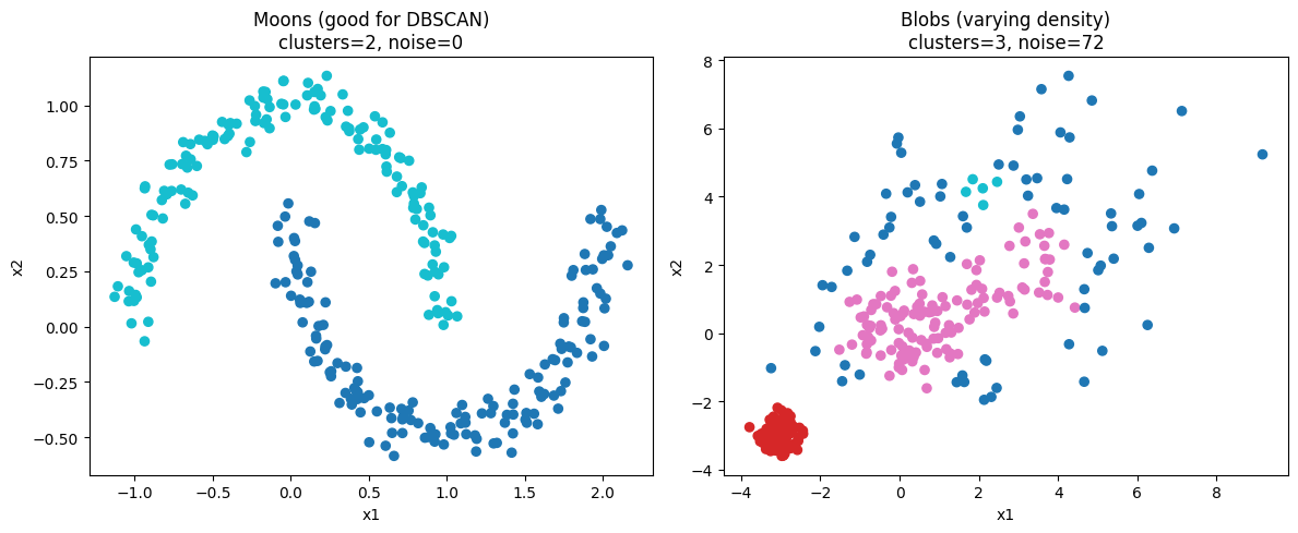
Results below.
Moons dataset: 2 clusters, 0 noise. Silhouette 0.3298. Davies–Bouldin 1.1514. ARI 1.0000. Blobs (varying density): 3 clusters, 72 noise points. Silhouette 0.3689. Davies–Bouldin 1.7966. ARI 0.5813.
Interpretation, short:
Silhouette near 0.3 indicates moderate cluster separation.
Lower Davies–Bouldin is better. Moons fit DBSCAN shape assumptions so metrics are strong and ARI is 1.0.
Blobs show many noise points and lower ARI. This reflects DBSCAN’s single global density assumption failing when clusters have different densities.
Would you like the code used or a version where I sweep eps and minPts and show metric trends?