Intiution

Intiution #

Imagine two classes of points in space. Many lines (or hyperplanes) could separate them.
SVM chooses the line that leaves the widest possible margin between the two classes.
The margin is defined by the support vectors: data points closest to the boundary.
Wider margin = better generalization to unseen data.
If data is not linearly separable, SVM uses the kernel trick to map it into higher dimensions where separation is possible.

Mathematical Formulation #

1. Linear SVM (Hard Margin)#

Given dataset: \((x_i, y_i)\), where \(x_i \in \mathbb{R}^n\), \(y_i \in \{-1, +1\}\).

We want a hyperplane:

\[ w \cdot x + b = 0 \]

where \(w\) is the weight vector, \(b\) is the bias.

Constraints (perfect separation):

\[ y_i (w \cdot x_i + b) \geq 1 \quad \forall i \]

Optimization (maximize margin = minimize norm of \(w\)):

\[ \min_{w,b} \; \frac{1}{2} \|w\|^2 \]

subject to above constraints.

2. Soft Margin SVM (with slack variables for misclassification)#

Allows some violations with penalty \(C\).

\[ \min_{w,b,\xi} \; \frac{1}{2} \|w\|^2 + C \sum_{i=1}^m \xi_i \]

subject to

\[ y_i (w \cdot x_i + b) \geq 1 - \xi_i, \quad \xi_i \geq 0 \]

Here:

\(C\) controls trade-off between large margin and classification errors.

3. Kernelized SVM (Non-linear)#

Use kernel function \(K(x_i, x_j)\) instead of explicit mapping \(\phi(x)\):

\[ K(x_i, x_j) = \phi(x_i) \cdot \phi(x_j) \]

Common kernels:

Linear: \(K(x_i, x_j) = x_i \cdot x_j\)
Polynomial: \(K(x_i, x_j) = (x_i \cdot x_j + 1)^d\)
RBF (Gaussian): \(K(x_i, x_j) = \exp(-\gamma \|x_i - x_j\|^2)\)

4. Dual Formulation #

The optimization can be expressed in terms of Lagrange multipliers \(\alpha_i\):

\[ \max_{\alpha} \sum_{i=1}^m \alpha_i - \frac{1}{2} \sum_{i=1}^m \sum_{j=1}^m \alpha_i \alpha_j y_i y_j K(x_i, x_j) \]

subject to

\[ \sum_{i=1}^m \alpha_i y_i = 0, \quad 0 \leq \alpha_i \leq C \]

Final classifier:

\[ f(x) = \text{sign}\left( \sum_{i=1}^m \alpha_i y_i K(x_i, x) + b \right) \]

# Demonstration of SVM intuition and math with toy datasets
# Three separate plots are produced:
# 1) Linearly separable data with a large C (close to hard-margin)
# 2) Same data with small C (soft margin, allows misclassification)
# 3) Non-linearly separable data handled by RBF kernel
#
# Rules followed:
# - Use matplotlib (no seaborn)
# - Each chart is a separate figure (no subplots)
# - No specific color settings are provided

import numpy as np
import matplotlib.pyplot as plt
from sklearn.datasets import make_blobs, make_circles
from sklearn.svm import SVC

fig, axes = plt.subplots(1, 3, figsize=(18, 6))

def plot_svm_subplot(ax, clf, X, y, title):
    ax.scatter(X[:, 0], X[:, 1], c=y, s=30)
    xlim = ax.get_xlim()
    ylim = ax.get_ylim()
    xx = np.linspace(xlim[0]-0.5, xlim[1]+0.5, 500)
    yy = np.linspace(ylim[0]-0.5, ylim[1]+0.5, 500)
    YY, XX = np.meshgrid(yy, xx)
    xy = np.vstack([XX.ravel(), YY.ravel()]).T
    if hasattr(clf, "decision_function"):
        Z = clf.decision_function(xy).reshape(XX.shape)
    else:
        Z = clf.predict_proba(xy)[:, 1].reshape(XX.shape)
    ax.contour(XX, YY, Z, levels=[-1.0, 0.0, 1.0],
               linestyles=['--','-','--'],
               linewidths=[1.0, 1.5, 1.0])
    sv = clf.support_vectors_
    ax.scatter(sv[:, 0], sv[:, 1], s=120, facecolors='none', linewidths=1.5)
    ax.set_title(title)
    ax.set_xlabel("Feature 1")
    ax.set_ylabel("Feature 2")
    ax.set_xlim(xlim)
    ax.set_ylim(ylim)
    ax.set_aspect('equal', adjustable='box')

# 1) Linearly separable data (hard-ish margin)
X1, y1 = make_blobs(n_samples=80, centers=2, cluster_std=0.6, random_state=2)
y1 = np.where(y1==0, -1, 1)  # convert labels to -1 and +1 for clarity

clf_hard = SVC(kernel='linear', C=10000000000)  # large C approximates hard margin
clf_hard.fit(X1, y1)

# 2) Same data but with soft margin (smaller C)
clf_soft = SVC(kernel='linear', C=0.001)  # allow misclassifications to increase margin
clf_soft.fit(X1, y1)

# 3) Non-linear data solved with RBF kernel
X2, y2 = make_circles(n_samples=200, factor=0.4, noise=0.08, random_state=1)
y2 = np.where(y2==0, -1, 1)

clf_rbf = SVC(kernel='rbf', gamma=5, C=1.0)
clf_rbf.fit(X2, y2)
plot_svm_subplot(axes[0], clf_hard, X1, y1, "Linear SVM (large C ≈ hard margin)")
plot_svm_subplot(axes[1], clf_soft, X1, y1, "Linear SVM (small C = soft margin)")
plot_svm_subplot(axes[2], clf_rbf, X2, y2, "RBF Kernel SVM (non-linear separation)")
plt.tight_layout()
plt.show()

# Print short explanation tying visuals to math
print("Interpretation:")
print(" - Decision boundary is where decision_function == 0.")
print(" - Support vectors lie on or near the margin lines (±1 for linear SVM).")
print(" - Large C forces fewer margin violations. It focuses on classification accuracy.")
print(" - Small C allows margin violations to increase margin width for better generalization.")
print(" - Kernel SVM uses an implicit mapping φ(x) so a linear boundary in feature space")
print("   corresponds to a non-linear boundary in the original input space.")

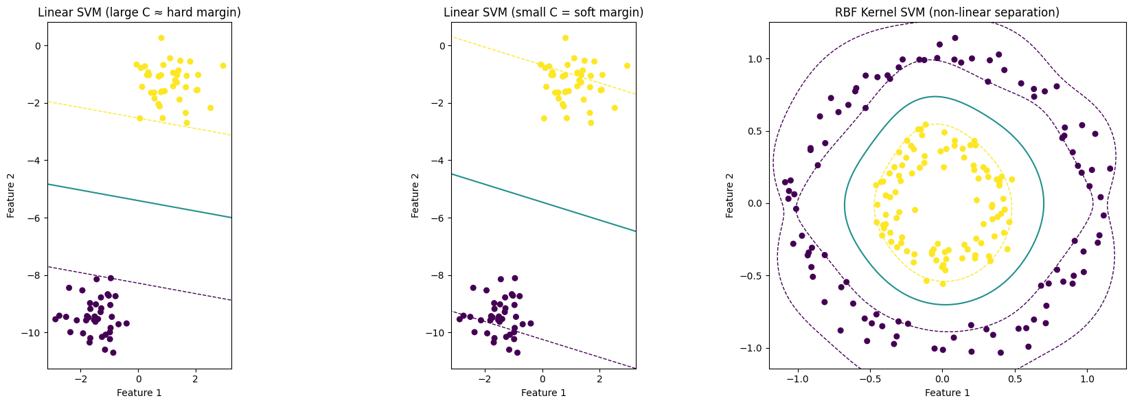
../../../_images/7615538893fa3ac22397ff4937f113d1be25898a8fc56f746668569523dfccb1.png

Interpretation:
 - Decision boundary is where decision_function == 0.
 - Support vectors lie on or near the margin lines (±1 for linear SVM).
 - Large C forces fewer margin violations. It focuses on classification accuracy.
 - Small C allows margin violations to increase margin width for better generalization.
 - Kernel SVM uses an implicit mapping φ(x) so a linear boundary in feature space
   corresponds to a non-linear boundary in the original input space.

Intiution

Contents

Intiution#

Mathematical Formulation#