How to select cluster \(k\)#
1. The Challenge#
If \(k\) is too small → clusters are too broad, losing detail.
If \(k\) is too large → clusters are too fragmented, may capture noise.
We need a method to balance fit and simplicity.
2. Methods to Select \(k\)#
A. Elbow Method#
Run K-Means with different \(k\) values (e.g., 1–10).
For each \(k\), calculate Within-Cluster Sum of Squares (WCSS):
\(C_i\) = cluster \(i\)
\(\mu_i\) = centroid of cluster \(i\)
Plot \(k\) vs WCSS.
Look for the “elbow point” where WCSS stops decreasing significantly.
This is usually the optimal \(k\).
Intuition: After this point, adding more clusters doesn’t reduce variance much.
B. Silhouette Score#
Measures how similar a point is to its own cluster vs other clusters.
\(a\) = average distance to points in the same cluster
\(b\) = average distance to points in the nearest other cluster
Range: -1 (bad) to 1 (good)
How to use:
Compute silhouette score for different \(k\) values.
Pick \(k\) with highest silhouette score.
C. Gap Statistic#
Compares the WCSS of your data with that of randomly generated data.
The optimal \(k\) is where your clustering is much better than random.
D. Domain Knowledge#
Sometimes, the optimal number of clusters is determined by business or scientific understanding.
Example: Customer segments, types of plants, or categories you already know exist.
E. Cross-validation (Optional)#
For advanced cases, you can use stability-based methods:
Split data
Run clustering
Check how consistently points are assigned
Higher stability → better \(k\)
3. Key Intuition#
You want clusters that are tight (points close to centroids) and well-separated (clusters far from each other).
Optimal \(k\) balances compactness and separation.
import numpy as np
import matplotlib.pyplot as plt
from sklearn.datasets import make_blobs
from sklearn.cluster import KMeans
from sklearn.metrics import silhouette_score
# Generate sample data
X, _ = make_blobs(n_samples=300, centers=4, cluster_std=0.60, random_state=42)
# Elbow Method
wcss = []
sil_scores = []
K = range(2, 11)
for k in K:
kmeans = KMeans(n_clusters=k, random_state=42)
kmeans.fit(X)
wcss.append(kmeans.inertia_) # WCSS
sil_scores.append(silhouette_score(X, kmeans.labels_))
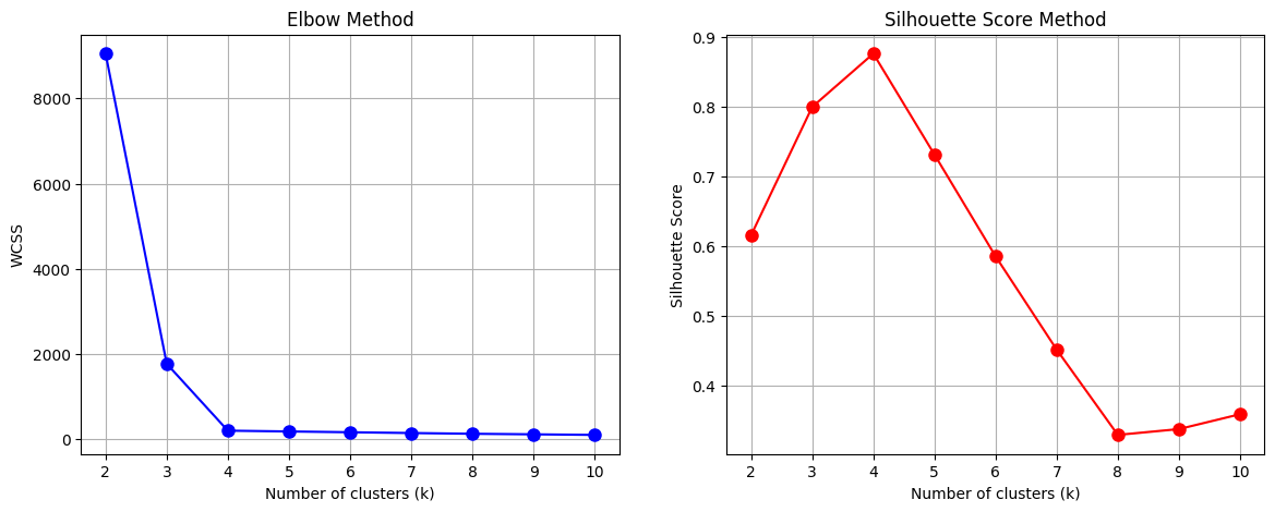
# Plot WCSS (Elbow Method)
plt.figure(figsize=(14, 5))
plt.subplot(1, 2, 1)
plt.plot(K, wcss, 'bo-', markersize=8)
plt.xlabel('Number of clusters (k)')
plt.ylabel('WCSS')
plt.title('Elbow Method')
plt.grid(True)
# Plot Silhouette Scores
plt.subplot(1, 2, 2)
plt.plot(K, sil_scores, 'ro-', markersize=8)
plt.xlabel('Number of clusters (k)')
plt.ylabel('Silhouette Score')
plt.title('Silhouette Score Method')
plt.grid(True)
plt.show()
import matplotlib.pyplot as plt
from sklearn.cluster import KMeans
from sklearn.metrics import silhouette_samples
import numpy as np
# Assume X is your data
k = 3
kmeans = KMeans(n_clusters=k, random_state=42)
labels = kmeans.fit_predict(X)
# Compute silhouette scores
sil_scores = silhouette_samples(X, labels)
y_lower = 0
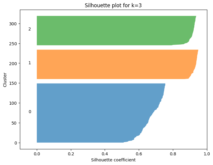
plt.figure(figsize=(8,6))
for i in range(k):
cluster_scores = sil_scores[labels == i]
cluster_scores.sort()
y_upper = y_lower + len(cluster_scores)
plt.fill_betweenx(np.arange(y_lower, y_upper),
0, cluster_scores,
alpha=0.7)
plt.text(-0.05, y_lower + len(cluster_scores)/2, str(i))
y_lower = y_upper + 10 # add gap between clusters
plt.xlabel("Silhouette coefficient")
plt.ylabel("Cluster")
plt.title(f"Silhouette plot for k={k}")
plt.xlim([-0.1, 1])
plt.show()
from sklearn.datasets import make_blobs
from sklearn.cluster import KMeans
from sklearn.metrics import silhouette_score, silhouette_samples
import matplotlib.pyplot as plt
import numpy as np
import warnings
warnings.filterwarnings("ignore")
# Generate sample data
X, _ = make_blobs(n_samples=300, centers=3, random_state=42)
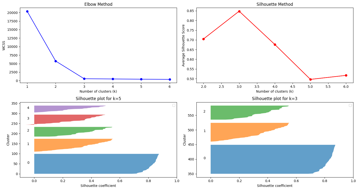
fig = plt.figure(figsize=(15, 8))
# Elbow Method
wcss = []
K = range(1, 7)
for k in K:
kmeans = KMeans(n_clusters=k, random_state=42)
kmeans.fit(X)
wcss.append(kmeans.inertia_)
ax1 = fig.add_subplot(221)
ax1.plot(K, wcss, 'bo-')
ax1.set_xlabel('Number of clusters (k)')
ax1.set_ylabel('WCSS')
ax1.set_title('Elbow Method')
# ax1.show()
# Silhouette Method
sil_scores = []
K = range(2, 7)
for k in K:
kmeans = KMeans(n_clusters=k, random_state=42)
labels = kmeans.fit_predict(X)
sil_scores.append(silhouette_score(X, labels))
ax2 = fig.add_subplot(222)
ax2.plot(K, sil_scores, 'ro-')
ax2.plot(K, sil_scores, 'ro-')
ax2.set_xlabel('Number of clusters (k)')
ax2.set_ylabel('Average Silhouette Score')
ax2.set_title('Silhouette Method')
# Assume X is your data
k = 5
kmeans = KMeans(n_clusters=k, random_state=42)
labels = kmeans.fit_predict(X)
# Compute silhouette scores
sil_scores = silhouette_samples(X, labels)
y_lower = 0
# plt.figure(figsize=(8,6))
ax3 = fig.add_subplot(223)
for i in range(k):
cluster_scores = sil_scores[labels == i]
cluster_scores.sort()
y_upper = y_lower + len(cluster_scores)
ax3.fill_betweenx(np.arange(y_lower, y_upper),
0, cluster_scores,
alpha=0.7)
ax3.text(-0.05, y_lower + len(cluster_scores)/2, str(i))
y_lower = y_upper + 10 # add gap between clusters
ax3.set_xlabel("Silhouette coefficient")
ax3.set_ylabel("Cluster")
ax3.set_title(f"Silhouette plot for k={k}")
ax3.set_xlim([-0.1, 1])
ax3.legend()
k=3
ax4 = fig.add_subplot(224)
for i in range(k):
cluster_scores = sil_scores[labels == i]
cluster_scores.sort()
y_upper = y_lower + len(cluster_scores)
ax4.fill_betweenx(np.arange(y_lower, y_upper),
0, cluster_scores,
alpha=0.7)
ax4.text(-0.05, y_lower + len(cluster_scores)/2, str(i))
y_lower = y_upper + 10 # add gap between clusters
ax4.set_xlabel("Silhouette coefficient")
ax4.set_ylabel("Cluster")
ax4.set_title(f"Silhouette plot for k={k}")
ax4.set_xlim([-0.1, 1])
ax4.legend()
plt.tight_layout()
plt.show()
1. Using the Elbow Method#
Step-by-Step Interpretation#
Plot WCSS (Within-Cluster Sum of Squares) vs number of clusters \(k\).
Look for the “elbow” point:
WCSS decreases sharply initially as clusters are added.
After some point, the decrease slows down → adding more clusters doesn’t improve much.
The elbow point is typically the optimal \(k\).
Intuition:
Before the elbow → adding clusters significantly reduces variance → meaningful separation.
After the elbow → diminishing returns → too many clusters may overfit.
Example (Hypothetical WCSS Plot)#
k |
WCSS |
|---|---|
1 |
1000 |
2 |
500 |
3 |
300 |
4 |
200 |
5 |
180 |
6 |
170 |
Sharp drop till k=3 → the elbow → choose k=3.
2. Using the Silhouette Curve#
Step-by-Step Interpretation#
For each \(k\), compute silhouette scores of all points.
Plot the silhouette curve (bars for each cluster).
Check:
Average silhouette score: higher is better (closer to 1).
Bar width: uniform bars indicate evenly distributed clusters.
Negative values: indicate misclassified points.
Intuition:
Large positive silhouette → cluster is tight and well-separated.
Small or negative silhouette → cluster overlaps with others → may need fewer/more clusters.
Example (Hypothetical Silhouette Scores)#
k |
Average Silhouette Score |
|---|---|
2 |
0.55 |
3 |
0.65 |
4 |
0.60 |
5 |
0.50 |
Highest score at k=3 → suggests k=3 clusters.
3. Combined Interpretation#
Method |
Observation |
Suggested k |
|---|---|---|
Elbow Method |
WCSS “elbow” at k=3 |
3 |
Silhouette Score |
Maximum average score at k=3 |
3 |
✅ Conclusion |
Both methods agree → optimal k = 3 |
3 |
Tip: Always consider both methods.
Elbow gives variance-based intuition.
Silhouette gives cohesion/separation intuition.
Interpretation from plots:
Find the elbow in the first plot → suggests a candidate \(k\).
Find maximum silhouette in the second plot → confirms the candidate.
Final \(k\) is where both methods agree.