Kernels#
A linear SVM works well if data is linearly separable.
But in many real-world problems, the boundary is nonlinear.
Kernel trick lets SVM map data into a higher-dimensional feature space without explicitly computing it.
This allows the SVM to learn nonlinear decision boundaries while still solving a linear optimization problem in that higher space.
📌 In simple words:
Without kernels: Draw a straight line in 2D.
With kernels: Map data to higher dimensions, then a straight line there looks like a curve back in 2D.
Common Types of Kernels#
(a) Linear Kernel#
Just the dot product of vectors.
No mapping, stays in the original space.
Best when data is linearly separable.
📌 Example use: Text classification (high-dimensional, sparse features).
(b) Polynomial Kernel#
Maps features into polynomial space of degree \(d\).
Can model curved decision boundaries.
📌 Example: Image recognition with curved boundaries.
(c) Radial Basis Function (RBF / Gaussian) Kernel#
Measures similarity: nearby points → high similarity; far points → low similarity.
Very flexible, can create complex nonlinear boundaries.
γ controls how far the influence of each point spreads.
📌 Example: Most common kernel, used when you don’t know the structure of data.
(d) Sigmoid Kernel#
Inspired by neural networks (acts like activation functions).
Not as commonly used as RBF.
📌 Example: Sometimes used in shallow neural-style problems.
3. Intuition with an Example#
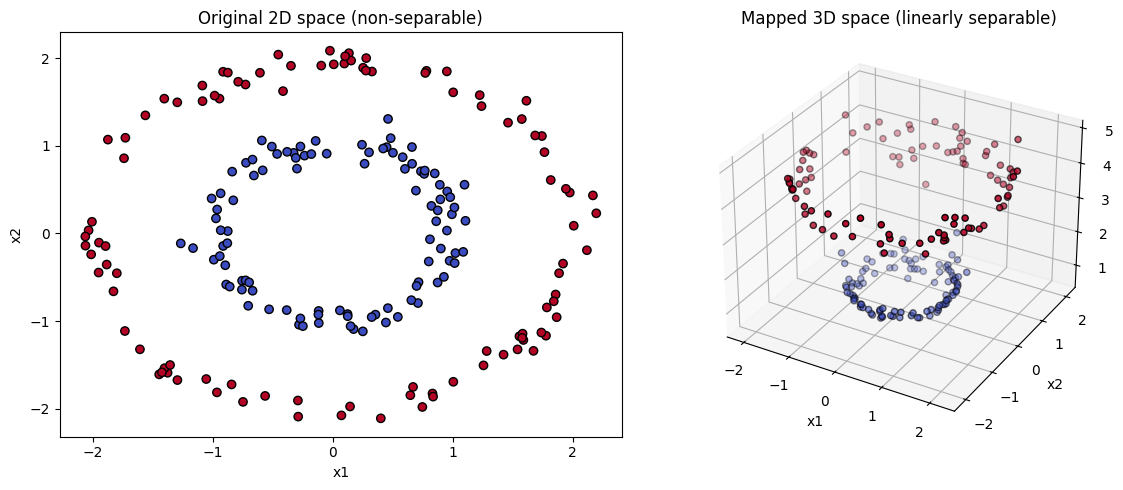
Imagine a dataset shaped like two concentric circles:
Linear SVM can’t separate them in 2D.
Apply RBF kernel → maps circles into higher-dimensional space where they become linearly separable.
So the kernel gives SVM power to handle nonlinearity.
4. Choosing a Kernel#
Linear → data roughly linearly separable, or very high-dimensional sparse data.
Polynomial → when interactions between features are important.
RBF → default choice, works well in most cases.
Sigmoid → niche, not commonly preferred.
In summary: Kernels = mathematical functions that let SVM project data into higher dimensions without explicitly transforming it, enabling nonlinear decision boundaries while keeping computations efficient.
import numpy as np
import matplotlib.pyplot as plt
from sklearn.datasets import make_moons
from sklearn.svm import SVC
# Generate nonlinear dataset (moons)
X, y = make_moons(n_samples=200, noise=0.2, random_state=42)
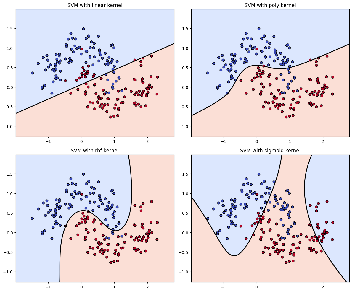
# Define kernels to compare
kernels = ["linear", "poly", "rbf", "sigmoid"]
models = [SVC(kernel=k, degree=3, gamma='scale').fit(X, y) for k in kernels]
# Create a mesh grid for plotting decision boundaries
xx, yy = np.meshgrid(np.linspace(X[:,0].min()-0.5, X[:,0].max()+0.5, 500),
np.linspace(X[:,1].min()-0.5, X[:,1].max()+0.5, 500))
plt.figure(figsize=(12, 10))
for i, (model, kernel) in enumerate(zip(models, kernels), 1):
Z = model.decision_function(np.c_[xx.ravel(), yy.ravel()])
Z = Z.reshape(xx.shape)
plt.subplot(2, 2, i)
plt.contourf(xx, yy, Z > 0, alpha=0.3, cmap=plt.cm.coolwarm)
plt.contour(xx, yy, Z, levels=[0], linewidths=2, colors='k')
plt.scatter(X[:,0], X[:,1], c=y, cmap=plt.cm.coolwarm, edgecolors='k')
plt.title(f"SVM with {kernel} kernel")
plt.tight_layout()
plt.show()
Linear SVM Geometry#
In standard SVM, the goal is to find the maximum-margin hyperplane that separates two classes.
Geometrically:
Each data point is represented as a vector in feature space.
The SVM finds a line (in 2D), plane (in 3D), or hyperplane (higher dims) that splits the data with largest margin.
👉 Works beautifully if the data is linearly separable.
What if the Data is Nonlinear?#
Example: two concentric circles (inner circle = class A, outer circle = class B).
In 2D, no straight line can separate them.
But if you map the data into higher dimensions:
Add a new feature \(z = x^2 + y^2\).
Now the circles become a line in 3D space, and a linear separator exists!
📌 Geometric trick: Make data “linearly separable” by lifting it into higher dimensions.
Kernel Trick — Geometry#
Here’s where kernels step in:
Instead of explicitly computing the high-dimensional mapping,
Kernels compute dot products in that higher space directly.
Geometrically:
A kernel function defines a new geometry of similarity between points.
Instead of “straight-line distance” in the original space, the kernel defines how “close” two points are in the transformed space.
The SVM then finds a linear hyperplane in that transformed space, which corresponds to a nonlinear boundary back in the original space.
Geometric Intuition for Common Kernels#
✅ Linear Kernel#
Geometry: Just the usual Euclidean geometry.
Hyperplane = straight line/plane.
✅ Polynomial Kernel#
Geometrically: Expands the space into all polynomial interactions up to degree \(d\).
A straight hyperplane in this expanded space = curved boundary in original space.
✅ RBF (Gaussian) Kernel#
Geometrically: Think of each point casting a “bump” of influence around it.
High γ → very tight bumps, decision boundary wiggles around data.
Low γ → wide bumps, boundary is smoother.
Essentially, it reshapes the geometry of distance: points far apart are almost orthogonal (unrelated).
✅ Sigmoid Kernel#
Geometrically: Similar to mapping into a neural network activation space.
Changes the angle/distance relationships into “S-shaped” similarity.
Intuitive Analogy#
Imagine the dataset as blobs of clay sitting on a flat table:
Linear SVM: Try to cut the clay with a knife in one straight slice.
Polynomial kernel: Bend the clay into curves and folds, then slice straight.
RBF kernel: Lift the clay into hills and valleys, then slice straight.
Sigmoid kernel: Pass clay through a squashing function before slicing.
So geometrically, kernels warp the space until a straight cut (hyperplane) becomes possible.
In summary:
Kernels redefine geometry by changing how we measure similarity.
This lets SVM carve complex boundaries by making the data look linear in some higher-dimensional space.
import numpy as np
import matplotlib.pyplot as plt
from mpl_toolkits.mplot3d import Axes3D

# Generate concentric circles dataset (nonlinear)
np.random.seed(42)
n_samples = 200
theta = 2 * np.pi * np.random.rand(n_samples)
r_inner = 1 + 0.1 * np.random.randn(n_samples//2)
r_outer = 2 + 0.1 * np.random.randn(n_samples//2)

X_inner = np.c_[r_inner * np.cos(theta[:n_samples//2]), r_inner * np.sin(theta[:n_samples//2])]
X_outer = np.c_[r_outer * np.cos(theta[n_samples//2:]), r_outer * np.sin(theta[n_samples//2:])]

X = np.vstack([X_inner, X_outer])
y = np.hstack([np.zeros(n_samples//2), np.ones(n_samples//2)])

# Polynomial mapping: z = x^2 + y^2
Z = np.sum(X**2, axis=1)

# ---- Plot original 2D space ----
plt.figure(figsize=(12,5))

plt.subplot(1,2,1)
plt.scatter(X[:,0], X[:,1], c=y, cmap=plt.cm.coolwarm, edgecolors='k')
plt.title("Original 2D space (non-separable)")
plt.xlabel("x1")
plt.ylabel("x2")

# ---- Plot transformed 3D space ----
ax = plt.subplot(1,2,2, projection='3d')
ax.scatter(X[:,0], X[:,1], Z, c=y, cmap=plt.cm.coolwarm, edgecolors='k')
ax.set_title("Mapped 3D space (linearly separable)")
ax.set_xlabel("x1")
ax.set_ylabel("x2")
ax.set_zlabel("x1² + x2²")

plt.tight_layout()
plt.show()