Local Outlier Factor

• Local Outlier Factor (LOF) is an unsupervised anomaly detection technique.

• Focuses on detecting local outliers — points that are unusual relative to their neighbors.

• Distinguishes between:

  • Local outlier: Close to a cluster but slightly different from neighbors.

  • Global outlier: Far from all clusters, clearly isolated.

---

2. Intuition Behind LOF

• LOF measures local density deviation:

  • Points in sparse regions compared to their neighbors → anomalies.

  • Uses k-nearest neighbors (kNN) to estimate local density.

• Key idea: Compare a point’s density with the density of its neighbors.

  • If density is much lower → point is a local outlier.

---

3. How LOF Works

1. Choose k, the number of nearest neighbors.

2. For each point:

   • Find its k nearest neighbors.

   • Compute the average distance to neighbors → estimates local density.

3. Compare local density of the point with densities of neighbors:

   • Low density relative to neighbors → high LOF score → outlier.

   • High density relative to neighbors → normal point.

• LOF score interpretation:

  • Score ≈ 1 → normal

  • Score > 1 → outlier

  • Higher score → stronger anomaly

---

4. Advantages

• Detects local anomalies that global methods (like Isolation Forest) might miss.

• Handles datasets with clusters of varying densities.

• Based on distance metrics: Euclidean, Manhattan, Minkowski, etc.

---

5. Practical Usage

• Available in sklearn.neighbors.LocalOutlierFactor.

• Parameters:

  • n_neighbors: Number of neighbors to use for density estimation.

  • metric: Distance metric (e.g., Euclidean, Manhattan).

  • contamination: Expected proportion of outliers.

• Output:

  • LOF score for each sample.

  • Can identify local anomalies for further analysis.

---

Summary

• LOF is useful for detecting local deviations in density.

• Especially effective when data has clusters with different densities.

• Uses k-nearest neighbor distances to compute local anomaly scores.

import numpy as np
import matplotlib.pyplot as plt
from sklearn.neighbors import LocalOutlierFactor

# Generate sample data
np.random.seed(42)
# Two clusters
cluster1 = np.random.randn(100, 2) + [2, 2]
cluster2 = np.random.randn(100, 2) + [7, 7]
# Outliers
outliers = np.array([[0, 0], [8, 0], [3, 9]])

# Combine data
X = np.vstack([cluster1, cluster2, outliers])

# Fit Local Outlier Factor
lof = LocalOutlierFactor(n_neighbors=20, contamination=0.05)  # 5% expected outliers
y_pred = lof.fit_predict(X)  # -1 = outlier, 1 = inlier
lof_scores = -lof.negative_outlier_factor_  # higher score = more anomalous

# Plot results
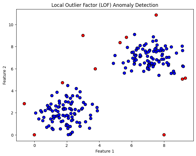
plt.figure(figsize=(8,6))
plt.scatter(X[:,0], X[:,1], c=['red' if i==-1 else 'blue' for i in y_pred], s=50, edgecolor='k')
plt.xlabel("Feature 1")
plt.ylabel("Feature 2")
plt.title("Local Outlier Factor (LOF) Anomaly Detection")
plt.show()

# Print outlier points
print("Detected outliers:")
print(X[y_pred==-1])

Detected outliers:
[[-0.6197451   2.8219025 ]
 [ 1.73534317  4.72016917]
 [ 7.51504769 10.85273149]
 [ 9.31465857  5.13273481]
 [ 3.75873266  5.97561236]
 [ 9.13303337  5.0479122 ]
 [ 5.67976679  8.83145877]
 [ 5.28686547  8.35387237]
 [ 0.          0.        ]
 [ 8.          0.        ]
 [ 3.          9.        ]]

Explanation

1. We generate two clusters and a few outliers.

2. LocalOutlierFactor computes LOF score for each sample based on k-nearest neighbors.

3. Points with low local density compared to neighbors are marked as outliers (-1).

4. We visualize:

   • Blue points → normal/inliers

   • Red points → detected outliers

---

Key Notes

• n_neighbors: Controls how “local” the density comparison is.

  • Small k → sensitive to local anomalies

  • Large k → more like global anomalies

• contamination: Expected fraction of anomalies, helps define threshold.

• LOF detects local anomalies that might not be far from other clusters but are sparse relative to their neighbors.