Intiution#
KNN is a lazy, instance-based algorithm used for classification and regression. Its core idea is:
“To predict the label of a new data point, look at the ‘k’ closest points in the training data and take a majority vote (for classification) or average (for regression).”
Think of it like this:
You move into a new neighborhood.
You want to know whether it’s mostly families or students living there.
You look at the nearest
khouses.If most of them are families, you conclude your house is likely in a family-dominated area.
Geometrical Intuition#
Data as points in space
Imagine every data sample as a point in an \(n\)-dimensional space (where \(n\) = number of features).
Example: If you have two features (height, weight), each person is a point in 2D plane.
Closeness = Similarity
When you want to predict a new point, you look at the nearest K neighbors.
“Nearness” is computed by a distance metric (Euclidean, Manhattan, cosine similarity, etc.).
Majority voting (classification)
If most of the nearest neighbors are of class “A”, the new point is classified as “A”.
Geometrically, this means:
The decision boundary between classes is formed by Voronoi regions (each point belongs to the region of its nearest training samples).
Averaging (regression)
If predicting a continuous value, the output is the average (or weighted average) of neighbor values.
Geometrically, this means you’re smoothing values across local neighborhoods.
Mathematical Intuition of KNN#
Suppose we want to predict the label \(\hat{y}\) of a new point \(x\).
1. Distance Computation#
For each training point \(x^{(i)}\):
This is Euclidean distance (but could be Manhattan, cosine, etc.).
2. Neighbor Selection#
Sort all training points by distance to \(x\).
Pick the K nearest points → call this set \(N_k(x)\).
3A. Classification Rule#
The predicted class is:
where:
\(\mathcal{C}\) = set of classes
\(\mathbf{1}(\cdot)\) = indicator function (1 if true, else 0)
It’s just majority voting.
If we use distance weighting (closer neighbors count more):
3B. Regression Rule#
The prediction is the average of neighbors:
Or, with distance weighting:
Summary
Geometrical view:
Data = points in space.
Predictions = decided by local neighbors.
Decision boundary = Voronoi regions.
Mathematical view:
Compute distances.
Select \(K\) neighbors.
Use majority vote (classification) or average (regression).
# Re-import required libraries after reset
import numpy as np
import matplotlib.pyplot as plt
from matplotlib.colors import ListedColormap
from sklearn.datasets import make_classification
from sklearn.neighbors import KNeighborsClassifier
# Generate synthetic dataset
X, y = make_classification(
n_samples=100, n_features=2, n_classes=2, n_redundant=0, n_clusters_per_class=1, random_state=42
)
# Fit KNN with K=5
knn = KNeighborsClassifier(n_neighbors=5)
knn.fit(X, y)
# Create meshgrid for decision boundary visualization
h = 0.02
x_min, x_max = X[:, 0].min() - 1, X[:, 0].max() + 1
y_min, y_max = X[:, 1].min() - 1, X[:, 1].max() + 1
xx, yy = np.meshgrid(np.arange(x_min, x_max, h), np.arange(y_min, y_max, h))
# Predictions for meshgrid
Z = knn.predict(np.c_[xx.ravel(), yy.ravel()])
Z = Z.reshape(xx.shape)
# Colors
cmap_light = ListedColormap(['#FFAAAA', '#AAAAFF'])
cmap_bold = ['#FF0000', '#0000FF']
# Plot decision boundary
plt.figure(figsize=(12, 6))
plt.contourf(xx, yy, Z, alpha=0.4, cmap=cmap_light)
# Plot training points
for idx, cl in enumerate(np.unique(y)):
plt.scatter(
X[y == cl, 0], X[y == cl, 1],
c=cmap_bold[idx], label=f"Class {cl}", edgecolor="k", s=60
)
# Pick a new test point
test_point = np.array([[0, 0]])
# Find neighbors
distances, indices = knn.kneighbors(test_point)
# Plot the test point
plt.scatter(test_point[:, 0], test_point[:, 1], c="gold", edgecolor="k", s=150, marker="*",
label="New Point")
# Plot neighbors with circles
for i in indices[0]:
plt.plot([test_point[0, 0], X[i, 0]], [test_point[0, 1], X[i, 1]], "k--", lw=1)
plt.scatter(X[i, 0], X[i, 1], s=200, facecolors='none', edgecolors='black', linewidth=2)
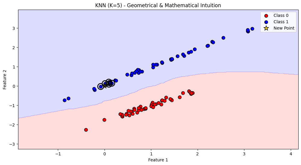
plt.title("KNN (K=5) - Geometrical & Mathematical Intuition")
plt.xlabel("Feature 1")
plt.ylabel("Feature 2")
plt.legend()
plt.show()