PCA#
Principal Component Analysis (PCA) is a dimensionality reduction technique that transforms high-dimensional data into a lower-dimensional space, while retaining as much variance (information) as possible.
Think of it as finding the “best perspective” to look at your data, where the structure or patterns are most visible.
Common uses:
Visualization (2D or 3D plots)
Noise reduction
Preprocessing for machine learning
Intuition Behind PCA#
Imagine you have 3D data points forming a thin, elongated cloud:
Most points vary along a diagonal direction.
The other two directions have very little spread (variance).
PCA identifies the direction of maximum variance (Principal Component 1), then the next orthogonal direction of maximum remaining variance (PC2), and so on.
By projecting data onto the top principal components:
You keep the most important information.
Ignore directions that contribute little (low variance → likely noise or redundancy).
Steps in PCA#
Standardize the data
Subtract the mean of each feature (centering) and scale to unit variance if features are on different scales.
Compute the covariance matrix
Measures how each pair of features varies together.
\[ \Sigma = \frac{1}{n-1} X^T X \]Compute eigenvectors and eigenvalues of covariance matrix
Eigenvectors = principal components (directions in feature space)
Eigenvalues = variance along each principal component
Sort eigenvectors by eigenvalues
Keep top \(k\) components that explain most variance (e.g., 95%)
Project original data onto these top components
This gives the reduced-dimensional representation:
\[ X_{reduced} = X \cdot W \]Where \(W\) is the matrix of top eigenvectors.
Mathematical Representation#
Original data: \(X \in \mathbb{R}^{n \times d}\) (n samples, d features)
Covariance matrix: \(\Sigma = \frac{1}{n-1} X^T X\)
Eigen decomposition: \(\Sigma v_i = \lambda_i v_i\)
\(v_i\) = eigenvector (principal component)
\(\lambda_i\) = eigenvalue (variance explained)
Dimensionality reduction: project onto top k eigenvectors with largest eigenvalues.
How PCA Reduces Dimensionality#
High-dimensional data often has correlated or redundant features.
PCA combines correlated features into principal components.
You keep only the most informative components → smaller feature space, less noise.
Example#
Suppose you have a dataset with 3 features:
Height, weight, and BMI
Height and weight are correlated → first principal component (PC1) might capture the “overall body size”
Second component (PC2) captures the small variation not explained by PC1
You could project your 3D data onto 2D (PC1 and PC2) and retain almost all variance.
Benefits of PCA#
Reduces dimensionality → faster computation
Removes noise → better model performance
Helps visualization in 2D/3D
Mitigates the curse of dimensionality
Limitations#
PCA is linear → may not capture non-linear relationships
Principal components are not always interpretable
Variance ≠ importance for predictive tasks → sometimes supervised feature selection is better
import numpy as np
import matplotlib.pyplot as plt
from mpl_toolkits.mplot3d import Axes3D
# Generate sample 3D data
np.random.seed(42)
n_samples = 100
mean = [0, 0, 0]
cov = [[3, 2, 0.5],
[2, 2, 0],
[0.5, 0, 1]]
X = np.random.multivariate_normal(mean, cov, n_samples)
# Compute PCA
X_meaned = X - np.mean(X, axis=0)
cov_matrix = np.cov(X_meaned.T)
eigenvalues, eigenvectors = np.linalg.eig(cov_matrix)
idx = np.argsort(eigenvalues)[::-1]
eigenvectors = eigenvectors[:, idx]
eigenvalues = eigenvalues[idx]
# Top 2 components for projection
W = eigenvectors[:, :2]
X_pca = X_meaned.dot(W)
# Plot 3D scatter and PCA vectors
fig = plt.figure(figsize=(12,6))
# 3D Scatter
ax = fig.add_subplot(121, projection='3d')
ax.scatter(X[:,0], X[:,1], X[:,2], alpha=0.6)
origin = np.mean(X, axis=0)
for i in range(2):
vec = eigenvectors[:,i] * 3 # scale for visibility
ax.quiver(origin[0], origin[1], origin[2],
vec[0], vec[1], vec[2],
color=['r','g'][i], linewidth=2, label=f'PC{i+1}')
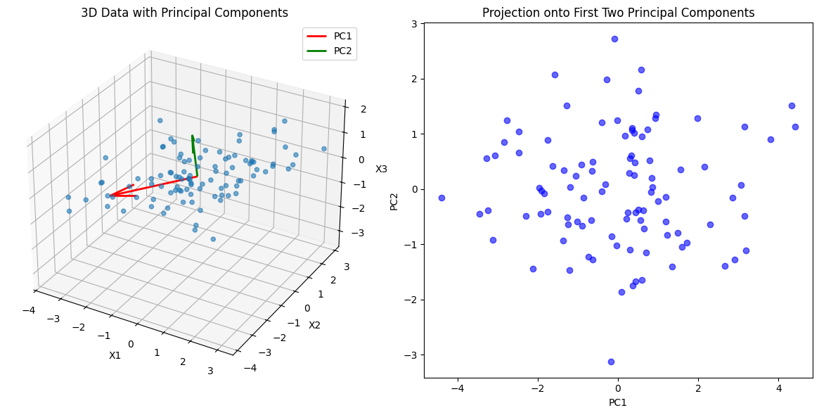
ax.set_title('3D Data with Principal Components')
ax.set_xlabel('X1')
ax.set_ylabel('X2')
ax.set_zlabel('X3')
ax.legend()
# 2D Projection
ax2 = fig.add_subplot(122)
ax2.scatter(X_pca[:,0], X_pca[:,1], alpha=0.6, color='b')
ax2.set_xlabel('PC1')
ax2.set_ylabel('PC2')
ax2.set_title('Projection onto First Two Principal Components')
plt.tight_layout()
plt.show()