OLS#
OLS (Ordinary Least Squares) is the most common method to estimate the parameters (coefficients) of a linear regression model.
It finds the best-fit line by minimizing the sum of squared errors (residuals) between actual and predicted values.
Objective#
OLS minimizes:
Where:
\(y_i\) = actual value
\(\hat{y}_i\) = predicted value
\(n\) = number of observations
This ensures the line is as close as possible to all data points.
Derivation (Simple Linear Regression)#
We solve for parameters \(\beta_0\) (intercept) and \(\beta_1\) (slope) using calculus:
Take partial derivatives of SSE wrt \(\beta_0\) and \(\beta_1\).
Set them = 0 (to minimize error).
Solve → gives the normal equations.
Final formulas:
Slope:
Intercept:
Multiple Linear Regression (Matrix Form)#
For multiple features:
OLS solution:
Where:
\(X\) = feature matrix
\(Y\) = target vector
\(\beta\) = coefficient vector
Why OLS?#
✅ Simple and widely used ✅ Provides exact solution (no iterations needed, unlike Gradient Descent) ✅ Works well when data assumptions hold (linearity, independence, homoscedasticity, normality of errors)
👉 In short: OLS gives us a mathematical way to find the regression line by minimizing squared differences between actual and predicted values.
import numpy as np
import matplotlib.pyplot as plt
import statsmodels.api as sm
# Generate synthetic linear data
np.random.seed(0)
X = np.linspace(0, 10, 50)
y = 3 + 2*X + np.random.normal(scale=3, size=X.shape)
# Add constant for intercept
X_with_const = sm.add_constant(X)
# Ordinary Least Squares regression
model = sm.OLS(y, X_with_const)
results = model.fit()
# Predictions
y_pred = results.predict(X_with_const)
# Plot
plt.figure(figsize=(10, 6))
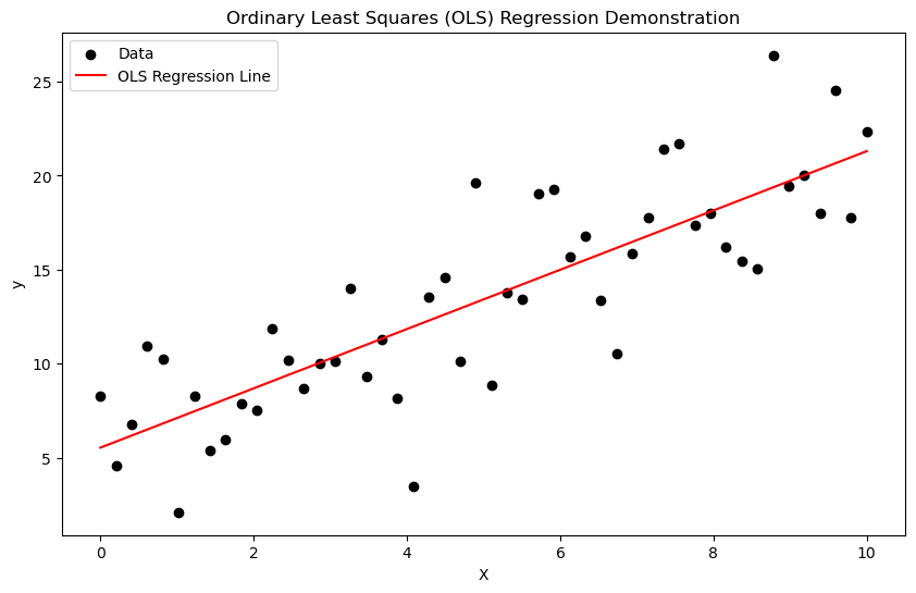
plt.scatter(X, y, label="Data", color="black")
plt.plot(X, y_pred, label="OLS Regression Line", color="red")
plt.xlabel("X")
plt.ylabel("y")
plt.title("Ordinary Least Squares (OLS) Regression Demonstration")
plt.legend()
plt.show()
# Display regression summary
print(results.summary())
                            OLS Regression Results
==============================================================================
Dep. Variable:                      y   R-squared:                       0.686
Model:                            OLS   Adj. R-squared:                  0.680
Method:                 Least Squares   F-statistic:                     105.1
Date:                Sat, 06 Sep 2025   Prob (F-statistic):           1.12e-13
Time:                        11:07:38   Log-Likelihood:                -128.12
No. Observations:                  50   AIC:                             260.2
Df Residuals:                      48   BIC:                             264.1
Df Model:                           1
Covariance Type:            nonrobust
==============================================================================
                 coef    std err          t      P>|t|      [0.025      0.975]
------------------------------------------------------------------------------
const          5.5391      0.892      6.207      0.000       3.745       7.333
x1             1.5765      0.154     10.252      0.000       1.267       1.886
==============================================================================
Omnibus:                        0.236   Durbin-Watson:                   2.078
Prob(Omnibus):                  0.889   Jarque-Bera (JB):                0.023
Skew:                          -0.051   Prob(JB):                        0.989
Kurtosis:                       3.022   Cond. No.                         11.7
==============================================================================

Notes:
[1] Standard Errors assume that the covariance matrix of the errors is correctly specified.
Interpretation of summary()#
Dep. Variable: y → The dependent variable being predicted. Here it’s
y.R-squared: 0.686 → 68.6% of the variation in
yis explained byx1. Decent explanatory power.Adj. R-squared: 0.680 → Adjusts for number of predictors. Very close to R² since only one predictor. Confirms good fit.
Model: OLS → Ordinary Least Squares regression used.
Method: Least Squares → Coefficients estimated by minimizing sum of squared residuals.
F-statistic: 105.1 → Tests whether the model explains significant variation in
y. Large value means strong relationship.Prob (F-statistic): 1.12e-13 → p-value for F-test. Almost zero. Model is statistically significant.
Date / Time → When the model was run. No analytical impact.
Log-Likelihood: -128.12 → Likelihood measure. Closer to 0 is better. Mainly used for comparing models.
AIC: 260.2 / BIC: 264.1 → Information criteria. Lower = better. Used when comparing models with different predictors.
Observations and Degrees of Freedom#
No. Observations: 50 → Sample size = 50. Larger samples give more reliable estimates.
Df Residuals: 48 → Degrees of freedom left after estimating parameters. Formula: \(n - k\), where \(k\) = number of estimated parameters (here 2: intercept + slope).
Df Model: 1 → Number of explanatory variables (only
x1).Covariance Type: nonrobust → Default error estimation. Alternatives (robust, clustered) handle heteroscedasticity or dependence.
Coefficients Table#
Variable |
Coefficient |
Std. Error |
t-Statistic |
P-Value |
95% Confidence Interval |
|---|---|---|---|---|---|
const |
5.5391 |
0.892 |
6.207 |
0.000 |
[3.745, 7.333] |
x1 |
1.5765 |
0.154 |
10.252 |
0.000 |
[1.267, 1.886] |
coef
const = 5.54→ Predicted \(y\) when \(x1 = 0\).x1 = 1.58→ For every 1-unit increase inx1,yincreases by ~1.58 units.
std err
Measures uncertainty of coefficient estimate. Smaller = more precise.
t
Test statistic for hypothesis \(H_0: \beta=0\).
Example: \(t = 10.25\) for
x1means the slope is very far from zero.
P>|t|
p-value for the t-test. Both are 0.000 → coefficients are statistically significant.
[0.025, 0.975]
95% confidence interval. For
x1, true slope lies between 1.27 and 1.89 with 95% confidence.
Residual Diagnostics#
Omnibus: 0.236 / Prob(Omnibus): 0.889 → Test for normality of residuals. High p-value = residuals look normal.
Jarque-Bera (JB): 0.023 / Prob(JB): 0.989 → Another normality test. p ≈ 0.99 → no evidence against normal distribution.
Skew: -0.051 → Residuals are almost symmetric (0 = perfect symmetry).
Kurtosis: 3.022 → Residuals have near-normal tail behavior (3 = normal).
Durbin-Watson: 2.078 → Tests autocorrelation in residuals. 2 = no autocorrelation. Value here is excellent.
Cond. No.: 11.7 → Condition number. Low (< 30) → no multicollinearity problems.
Impact Summary#
Model is statistically significant (F-test p ≈ 0).
x1 strongly predicts
y(slope ~1.58, highly significant).Residual diagnostics confirm assumptions of OLS hold (normality, independence, no multicollinearity).
About 69% of variation in
yis explained. Remaining 31% is due to noise or omitted variables.
DIfference between OLS & Gradient Descent#
Ordinary Least Squares (OLS)#
Definition: A closed-form analytical solution to find regression coefficients (β) that minimize the sum of squared residuals (errors).
Formula:
\[ \hat{\beta} = (X^TX)^{-1}X^Ty \]where \(X\) = features matrix, \(y\) = target vector.
Characteristics:
Direct computation, no iteration.
Fast for small datasets with few features.
Requires computing the inverse of \(X^TX\), which can be expensive if the dataset has very high dimensionality.
Works best when features are not highly correlated (multicollinearity can cause instability).
Gradient Descent (GD)#
Definition: An iterative optimization algorithm that minimizes the cost function (e.g., Mean Squared Error) by gradually updating coefficients in the opposite direction of the gradient.
Update rule:
\[ \beta_j := \beta_j - \alpha \frac{\partial J(\beta)}{\partial \beta_j} \]where \(\alpha\) = learning rate.
Characteristics:
Works even when closed-form solutions are not feasible (e.g., large-scale data, complex models).
Handles very high-dimensional data efficiently since it avoids matrix inversion.
Requires choosing hyperparameters (learning rate, iterations).
May converge slowly or get stuck in local minima (for non-convex problems).
Key Differences
Aspect |
OLS (Closed-form) |
Gradient Descent (Iterative) |
|---|---|---|
Solution type |
Exact (analytical) |
Approximate (iterative) |
Computation |
Requires matrix inversion \((X^TX)^{-1}\) |
Updates step by step using gradients |
Speed |
Fast for small/medium datasets |
Scales better for huge datasets |
Memory |
Needs to store large matrices |
Works in batches (mini-batch GD) |
Use case |
Low-dimensional, small data |
Large-scale, high-dimensional, online learning |
Summary:
Use OLS when the dataset is small, with few features → quick and exact.
Use Gradient Descent when the dataset is very large or high-dimensional → scalable and flexible.