Cost Function#
AdaBoost doesn’t use Mean Squared Error (MSE) or cross-entropy directly. Instead, it optimizes an exponential loss function, which is tightly linked to how weights and classifier contributions are updated.
1. Exponential Loss as the Cost Function#
For binary classification, let:
True labels: \(y_i \in \{-1, +1\}\)
Strong classifier output:
\[ f(x) = \sum_{t=1}^T \alpha_t h_t(x) \]where \(h_t(x)\) is the weak learner’s prediction and \(\alpha_t\) is its weight.
The AdaBoost loss function is:
🔍 Intuition:#
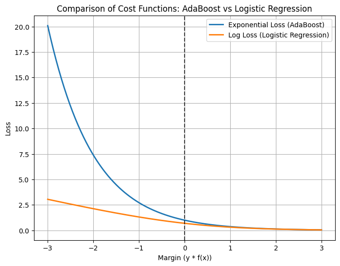
If \(y_i f(x_i)\) is positive and large → prediction is correct with high confidence → loss is small (\(e^{-\text{large}}\)).
If \(y_i f(x_i)\) is negative → misclassified → loss grows exponentially.
👉 This makes AdaBoost very sensitive to misclassified points (and outliers).
2. Weighted Error Minimization#
At each iteration, AdaBoost minimizes a weighted classification error:
This connects to the exponential loss because updating weights:
is exactly the gradient-descent step for minimizing exponential loss.
3. Cost Function in Terms of Margins#
The margin for a point is:
Large positive margin → correct and confident classification.
Negative margin → misclassification.
AdaBoost implicitly maximizes the margin by minimizing exponential loss. This is why its decision boundary often looks similar to an SVM boundary.
Summary
AdaBoost cost function = Exponential Loss:
\[ L = \sum_{i=1}^n e^{-y_i f(x_i)} \]Misclassified points incur huge penalties, so the algorithm shifts focus toward them.
The cost function ties directly to:
Learner weights (\(\alpha_t = \tfrac{1}{2} \ln\frac{1-\epsilon_t}{\epsilon_t}\))
Sample weight updates (increase weight of misclassified points).
Geometric interpretation: AdaBoost minimizes exponential loss ≈ maximizes the margin.
import numpy as np
import matplotlib.pyplot as plt
from sklearn.datasets import make_classification
from sklearn.ensemble import AdaBoostClassifier
from sklearn.tree import DecisionTreeClassifier
from sklearn.linear_model import LogisticRegression

# Generate binary classification dataset
X, y = make_classification(
    n_samples=200, n_features=2, n_redundant=0, n_informative=2,
    n_clusters_per_class=1, class_sep=1.2, random_state=42
)

# Train AdaBoost
ada = AdaBoostClassifier(
    estimator=DecisionTreeClassifier(max_depth=1),
    n_estimators=50, random_state=42
)
ada.fit(X, y)

# Train Logistic Regression (for comparison with log loss)
log_reg = LogisticRegression()
log_reg.fit(X, y)

# Compute margins (y*f(x)) for AdaBoost
f_scores = np.sum([estimator.predict(X) * alpha
                   for estimator, alpha in zip(ada.estimators_, ada.estimator_weights_)], axis=0)
margins = y * f_scores

# Exponential loss for AdaBoost
exp_loss = np.exp(-margins)

# Logistic loss for comparison
logits = log_reg.decision_function(X)
log_loss = np.log(1 + np.exp(-y * logits))

# Plot losses vs margins
m = np.linspace(-3, 3, 200)
exp_curve = np.exp(-m)
log_curve = np.log(1 + np.exp(-m))

plt.figure(figsize=(8,6))
plt.plot(m, exp_curve, label="Exponential Loss (AdaBoost)", linewidth=2)
plt.plot(m, log_curve, label="Log Loss (Logistic Regression)", linewidth=2)
plt.axvline(x=0, color='k', linestyle='--', alpha=0.7)
plt.xlabel("Margin (y * f(x))")
plt.ylabel("Loss")
plt.title("Comparison of Cost Functions: AdaBoost vs Logistic Regression")
plt.legend()
plt.grid(True)
plt.show()