Cost Functions#
t-SNE tries to match the similarity between points in high-dimensional space with their similarity in low-dimensional space.
High-dimensional points → similarity probabilities \(p_{ij}\)
Low-dimensional embedding → similarity probabilities \(q_{ij}\)
The cost function measures the difference between these two distributions.
2. High-Dimensional Similarities#
For points \(x_i\) and \(x_j\) in high-dimensional space:
Conditional probability that \(x_i\) picks \(x_j\) as neighbor.
\(\sigma_i\) is chosen so that perplexity matches the desired neighborhood size.
Symmetrize:
Ensures the similarity measure is symmetric.
3. Low-Dimensional Similarities#
For low-dimensional points \(y_i\) and \(y_j\):
Uses Student-t distribution (heavy-tailed) to allow distant points to spread out.
This addresses the crowding problem, which occurs when projecting high-D data to 2D/3D.
4. Cost Function (KL Divergence)#
t-SNE minimizes the Kullback-Leibler (KL) divergence between the high-D and low-D distributions:
Interpretation:
High \(p_{ij}\) → points are close in high-D space → want \(q_{ij}\) to also be high.
If \(q_{ij}\) is too low → contributes a large term to KL → gradient will pull points closer.
Gradient descent is used to iteratively minimize \(C\) and adjust the low-dimensional points \(y_i\).
5. Intuition#
Concept |
Intuition |
|---|---|
\(p_{ij}\) |
How similar points are in high-D |
\(q_{ij}\) |
How similar points are in low-D embedding |
KL divergence |
Penalizes mismatch between high-D and low-D similarity |
Minimization |
Moves points so that neighbors stay close and non-neighbors are separated |
Think of t-SNE as adjusting points in 2D/3D so that the “neighborhoods” of points in high-D space are preserved.
6. Key Notes#
Focus on Local Structure
KL divergence gives more weight to small \(p_{ij}\) errors → preserves local neighborhoods.
Heavy-tailed Distribution
Prevents distant points from collapsing into the center of the embedding.
Non-linear Optimization
The cost function is non-convex → multiple runs may yield slightly different embeddings.
import numpy as np
import matplotlib.pyplot as plt
from sklearn.datasets import make_blobs
from sklearn.manifold import TSNE
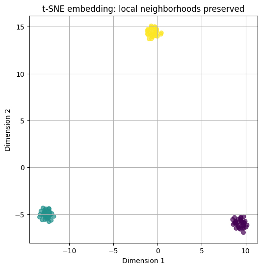
# Step 1: Generate synthetic 5D data with 3 clusters
X, y = make_blobs(n_samples=100, centers=3, n_features=5, random_state=42)
# Step 2: Initialize t-SNE
tsne = TSNE(n_components=2, perplexity=30, random_state=42)
# Step 3: Fit and transform data
X_embedded = tsne.fit_transform(X)
# Step 4: Plot the low-dimensional embedding
plt.figure(figsize=(6, 6))
plt.scatter(X_embedded[:, 0], X_embedded[:, 1], c=y, cmap='viridis', alpha=0.7)
plt.title("t-SNE embedding: local neighborhoods preserved")
plt.xlabel("Dimension 1")
plt.ylabel("Dimension 2")
plt.grid(True)
plt.show()