Isolation Forest#
Isolation Forest (iForest) is an unsupervised machine learning algorithm for anomaly detection.
Goal: Identify outliers (anomalies) in the data.
Key idea: Anomalies are easier to isolate than normal points.
Works well for high-dimensional data and large datasets.
It does not rely on distance or density like KNN or DBSCAN. Instead, it isolates points using random splits.
2. Intuition Behind Isolation Forest#
Imagine a dataset with normal points forming dense clusters and anomalies scattered far away.
Isolation Forest isolates points recursively using random splits:
Normal points require more splits to isolate (they’re in dense regions).
Anomalies require fewer splits to isolate (they’re far from other points).
Think of it as chopping a tree:
Dense regions → deeper branches
Outliers → isolated in shallow branches
3. How It Works (Step-by-Step)#
Build Isolation Trees:
Randomly select a feature.
Randomly select a split value between the min and max of that feature.
Partition data into two subsets.
Repeat recursively until:
Each point is isolated, or
Maximum tree depth is reached.
Compute Path Length:
Path length \(h(x)\) = number of splits needed to isolate point \(x\) in a tree.
Anomalies → short path length
Normal points → long path length
Repeat for Multiple Trees:
Build an ensemble of isolation trees (like a forest) to reduce variance.
Average path lengths across all trees.
Compute Anomaly Score:
Where:
\(E(h(x))\) = average path length of \(x\) across trees
\(c(n)\) = average path length in a binary search tree of \(n\) points (normalization)
Interpretation:
\(s(x) \approx 1\) → anomaly
\(s(x) \approx 0.5\) → normal
\(s(x) < 0.5\) → likely normal
4. Parameters in Isolation Forest#
Parameter |
Description |
|---|---|
|
Number of isolation trees in the forest |
|
Number of samples to draw for each tree |
|
Expected proportion of anomalies (used to set threshold) |
|
Number of features to consider when splitting |
|
Seed for reproducibility |
5. Advantages#
Efficient and scalable (linear time complexity \(O(n \log n)\))
Works with high-dimensional data
No assumption about data distribution
Handles both global and local anomalies
6. Python Example#
import numpy as np
import matplotlib.pyplot as plt
from sklearn.ensemble import IsolationForest

# Example data
X = np.random.randn(300, 2)  # normal points
X = np.vstack([X, [[5, 5], [6, 6]]])  # anomalies

# Fit Isolation Forest
clf = IsolationForest(contamination=0.05, random_state=42)
clf.fit(X)
y_pred = clf.predict(X)  # 1 = normal, -1 = anomaly

# Plot
plt.scatter(X[:,0], X[:,1], c=['red' if i==-1 else 'blue' for i in y_pred])
plt.xlabel("Feature 1")
plt.ylabel("Feature 2")
plt.title("Isolation Forest Anomaly Detection")
plt.show()
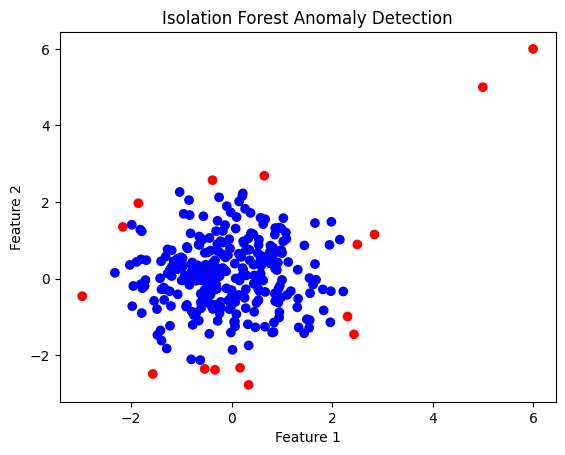
✅ Blue points → normal, red points → anomalies
7. Summary#
Isolation Forest isolates anomalies rather than profiling normal points.
Outliers are separated quickly (short path), normal points slowly (long path).
Uses multiple trees for robustness.
Generates an anomaly score to classify points.