SVR#
Support Vector Regression (SVR) is an application of Support Vector Machines (SVM) for regression problems.
Instead of predicting class labels, SVR predicts continuous values.
The key idea: SVR tries to fit a function that approximates the data, while keeping errors within a certain tolerance.
The Core Idea (ε-insensitive Tube)#
SVR introduces the concept of an ε-tube:
Predictions within ±ε from the true value are considered “good enough” → no penalty.
Only predictions outside this tube contribute to the error.
Mathematical Formulation#
We want to find a function:
that predicts targets \(y\) given features \(x\).
Optimization Problem:#
subject to:
Explanation of Terms:#
\(\frac{1}{2}\|w\|^2\): margin maximization (flatness of the function).
\(C\): regularization parameter, controls penalty for points outside the tube.
\(\epsilon\): tube width, tolerance for error.
\(\xi_i, \xi_i^*\): slack variables, measure deviations beyond ε.
\(\phi(x)\): kernel mapping.
Hyperparameters in SVR#
C → Regularization (trade-off between flatness vs tolerance to errors).
ε (epsilon) → Size of the ε-tube. Larger ε → simpler model, fewer support vectors.
γ (gamma) → Kernel coefficient (in RBF, controls influence of single points).
Kernels in SVR#
Just like SVC, SVR can use different kernels:
Linear: best for linear data.
RBF (default): captures nonlinear relationships.
Polynomial: fits polynomial curves.
Example in Python (Scikit-learn)#
import numpy as np
import matplotlib.pyplot as plt
from sklearn.svm import SVR
# Generate toy dataset
X = np.sort(5 * np.random.rand(40, 1), axis=0)
y = np.sin(X).ravel()
y[::5] += 3 * (0.5 - np.random.rand(8)) # add noise
# Define SVR models
svr_rbf = SVR(kernel='rbf', C=100, gamma=0.1, epsilon=0.1)
svr_lin = SVR(kernel='linear', C=100, epsilon=0.1)
svr_poly = SVR(kernel='poly', C=100, degree=3, epsilon=0.1)
# Fit
y_rbf = svr_rbf.fit(X, y).predict(X)
y_lin = svr_lin.fit(X, y).predict(X)
y_poly = svr_poly.fit(X, y).predict(X)
# Plot
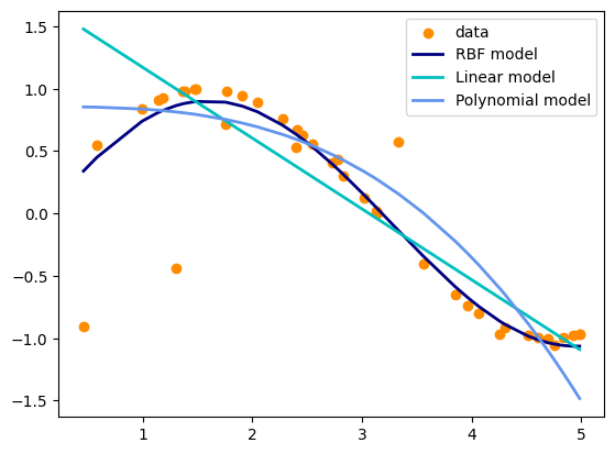
plt.scatter(X, y, color='darkorange', label='data')
plt.plot(X, y_rbf, color='navy', lw=2, label='RBF model')
plt.plot(X, y_lin, color='c', lw=2, label='Linear model')
plt.plot(X, y_poly, color='cornflowerblue', lw=2, label='Polynomial model')
plt.legend()
plt.show()
Key Takeaways
SVR tries to keep predictions within an ε-tube around the true values.
C → controls penalty for errors outside ε.
ε → defines tolerance zone for errors.
γ → controls influence range of training points in nonlinear kernels.
Flexible → can capture both linear and nonlinear regression patterns