Cost Function#
1. Gradient Boosting Regressor (GBR)#
Purpose: Minimize prediction error for continuous targets.
Common Loss Functions:#
Mean Squared Error (MSE)
Measures squared differences between predicted and true values.
Gradient w.r.t prediction:
Pseudo-residuals: \(r_i = y_i - \hat{y}_i\) → what each tree fits.
Mean Absolute Error (MAE)
More robust to outliers.
Gradient:
Trees fit the direction of error instead of squared magnitude.
Huber Loss (Combination of MSE & MAE)
Smooth near zero, linear for large errors → robust and stable.
Workflow for GBR:
Compute pseudo-residuals: negative gradient of chosen loss.
Fit tree to residuals.
Update model: \(F_m = F_{m-1} + \nu \gamma_m h_m(x)\).
2. Gradient Boosting Classifier (GBC)#
Purpose: Minimize prediction error for categorical targets.
Common Loss Functions:#
Binary Cross-Entropy / Log Loss
\(y_i \in \{0,1\}\), \(\hat{p}_i = \sigma(F(x_i))\)
Negative gradient (pseudo-residuals):
Each tree tries to fit \(r_i\) → improves probability estimates.
Multiclass Cross-Entropy
\(y_{ik} = 1\) if sample \(i\) belongs to class \(k\), else 0.
\(\hat{p}_{ik} = \text{softmax}(F_k(x_i))\)
Pseudo-residuals for each class:
Trees are trained per class to fit residuals.
Intuition
GBR: Loss is continuous → residual = actual - predicted.
GBC: Loss is probabilistic → residual = observed probability - predicted probability.
Gradient boosting fits a tree to the negative gradient of the loss in every iteration.
Choice of loss determines robustness, sensitivity to outliers, and type of problem.
import numpy as np
import matplotlib.pyplot as plt
from sklearn.tree import DecisionTreeRegressor
from sklearn.datasets import make_classification
from sklearn.preprocessing import LabelBinarizer
from scipy.special import expit # sigmoid
import warnings
warnings.filterwarnings("ignore")
# -------------------------------
# Part 1: Gradient Boosting Regressor (GBR)
# -------------------------------
# Dataset
X_reg = np.linspace(0, 10, 10).reshape(-1,1)
y_reg = np.array([1.5, 1.7, 3.2, 3.9, 5.1, 5.8, 7.0, 7.9, 9.2, 10.1])
# Initialize prediction (F0)
F0 = np.mean(y_reg)
Fm = np.full_like(y_reg, F0, dtype=float)
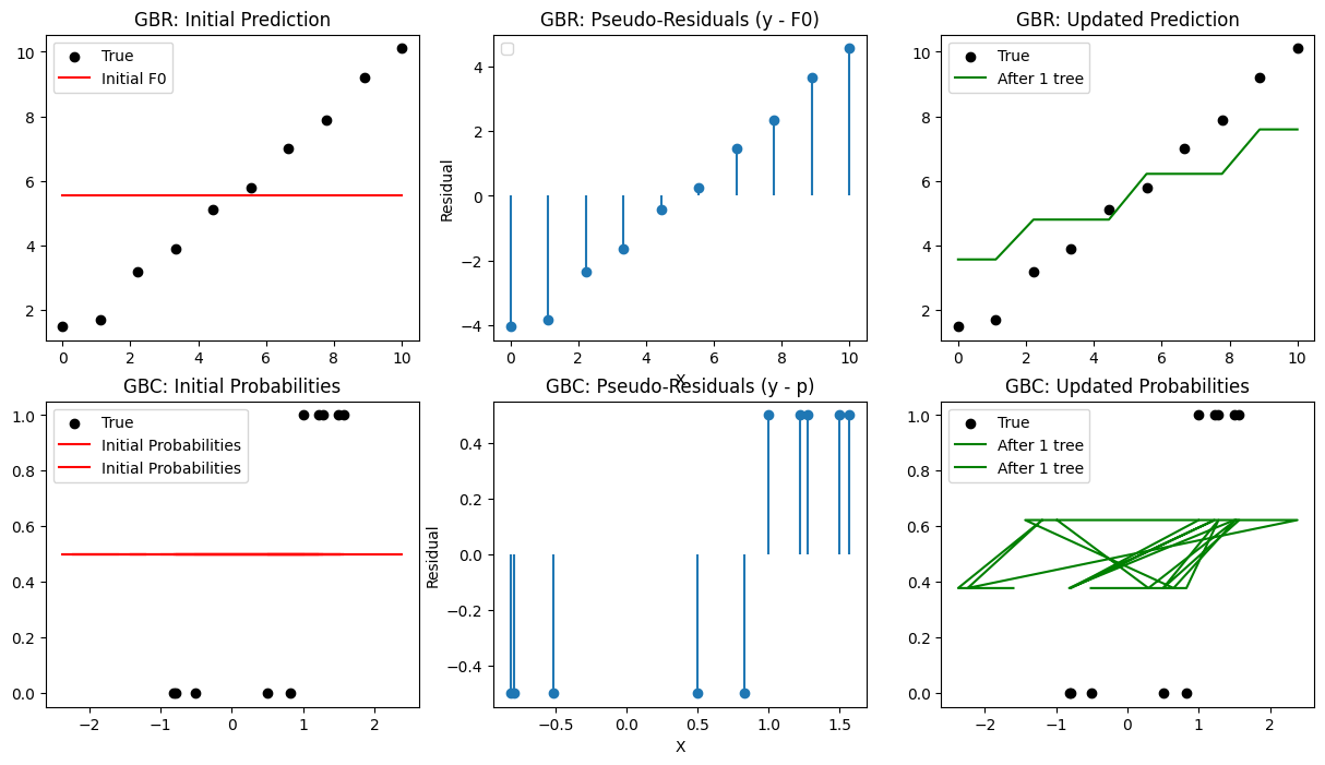
plt.figure(figsize=(15,8))
plt.subplot(2,3,1)
plt.scatter(X_reg, y_reg, color='black', label='True')
plt.plot(X_reg, Fm, color='red', label='Initial F0')
plt.title("GBR: Initial Prediction")
plt.legend()
# Compute pseudo-residuals (MSE)
residuals = y_reg - Fm
plt.subplot(2,3,2)
plt.stem(X_reg, residuals, basefmt=" ")
plt.title("GBR: Pseudo-Residuals (y - F0)")
plt.xlabel("X")
plt.ylabel("Residual")
plt.legend()
# Fit a weak learner
tree = DecisionTreeRegressor(max_depth=2)
tree.fit(X_reg, residuals)
pred = tree.predict(X_reg)
Fm += 0.5 * pred # learning_rate=0.5
plt.subplot(2,3,3)
plt.scatter(X_reg, y_reg, color='black', label='True')
plt.plot(X_reg, Fm, color='green', label='After 1 tree')
plt.title("GBR: Updated Prediction")
plt.legend()
# -------------------------------
# Part 2: Gradient Boosting Classifier (GBC)
# -------------------------------
# Binary classification dataset
X_clf, y_clf = make_classification(
n_samples=10,
n_features=2, # must be >= log2(n_classes*n_clusters_per_class)
n_informative=2,
n_redundant=0,
n_repeated=0,
n_classes=2,
random_state=0
)
y_clf = y_clf.reshape(-1,1)
# Initialize prediction (F0 for log-odds)
p0 = np.mean(y_clf)
F0 = np.log(p0/(1-p0))
Fm = np.full_like(y_clf, F0, dtype=float)
# Compute pseudo-residuals
p = expit(Fm) # sigmoid probabilities
residuals = y_clf - p
plt.subplot(2,3,4)
plt.scatter(X_clf[:,0], y_clf, color='black', label='True')
plt.plot(X_clf, p, color='red', label='Initial Probabilities')
plt.title("GBC: Initial Probabilities")
plt.legend()
plt.subplot(2,3,5)
plt.stem(X_clf[:,0], residuals, basefmt=" ")
plt.title("GBC: Pseudo-Residuals (y - p)")
plt.xlabel("X")
plt.ylabel("Residual")
# Fit weak learner
tree = DecisionTreeRegressor(max_depth=2)
tree.fit(X_clf, residuals)
pred = tree.predict(X_clf)
Fm = Fm.flatten() # shape (10,)
pred = pred.flatten() # shape (10,)
Fm += 0.5 * pred # works
Fm += 0.5 * pred # learning_rate=0.5
p = expit(Fm)
plt.subplot(2,3,6)
plt.scatter(X_clf[:,0], y_clf, color='black', label='True')
plt.plot(X_clf, p, color='green', label='After 1 tree')
plt.title("GBC: Updated Probabilities")
plt.legend()
plt.show()