Overview#
Simple linear regression is a supervised machine learning technique for regression tasks. It uses a dataset with known inputs and outputs to learn a model that predicts a continuous value for new inputs.
Core Idea#
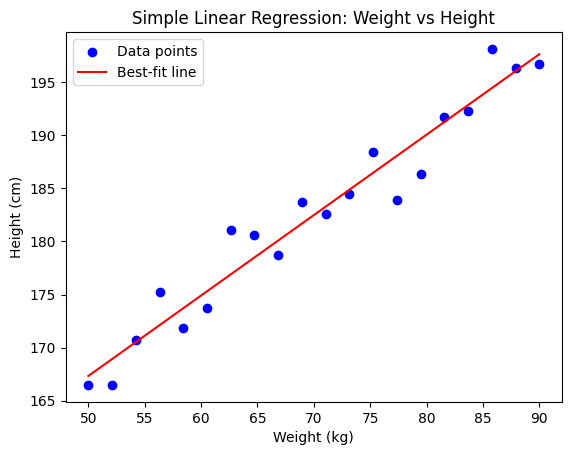
The goal is to find a best-fit line through the data that minimizes the error between predictions and actual values. This line shows the relationship between:
Independent variable (x) → input feature (e.g., weight)
Dependent variable (y) → output (e.g., height)
Hypothesis Function#
The prediction is represented by a linear equation:
\(x\): input feature
\(h_\theta(x)\): predicted output
\(\theta_0\): intercept (value when \(x=0\))
\(\theta_1\): slope (how much \(y\) changes when \(x\) increases by 1)
Training means finding the best values of \(\theta_0\) and \(\theta_1\).
Cost Function (Error Measurement)#
To measure fit, we use the Mean Squared Error (MSE):
\(m\): number of data points
\(x^{(i)}, y^{(i)}\): i-th input and true output
Squared error ensures all errors are positive and penalizes large deviations
Objective: minimize \(J(\theta_0, \theta_1)\).
Gradient Descent (Optimization)#
To minimize the cost function, we use gradient descent. It iteratively adjusts parameters in the direction that reduces error:
\(\alpha\): learning rate (step size)
\(\frac{\partial}{\partial \theta_j} J\): derivative (slope) of the cost function w.r.t. parameter \(\theta_j\)
Update Rules#
By expanding the derivatives, we get:
Intercept update:
Slope update:
These updates repeat until convergence at the global minimum of the cost function, giving the best-fit line.
import numpy as np
import matplotlib.pyplot as plt

# Generate sample dataset (weight vs height)
np.random.seed(42)
weights = np.linspace(50, 90, 20)   # weights (kg)
heights = 0.9 * weights + 120 + np.random.randn(20) * 3  # linear relation with noise

# Scatter plot of dataset
plt.scatter(weights, heights, color="blue", label="Data points")

# Linear Regression using closed-form solution (Normal Equation)
X = np.c_[np.ones(weights.shape[0]), weights]  # add bias term
theta_best = np.linalg.inv(X.T @ X) @ X.T @ heights  # (X^T X)^-1 X^T y

# Predicted line
line_x = np.linspace(50, 90, 100)
line_y = theta_best[0] + theta_best[1] * line_x

plt.plot(line_x, line_y, color="red", label="Best-fit line")

# Labels
plt.title("Simple Linear Regression: Weight vs Height")
plt.xlabel("Weight (kg)")
plt.ylabel("Height (cm)")

plt.legend()
plt.show()
Assumptions#
Linear regression looks deceptively simple—fit a straight line, done! But under the hood, it quietly relies on a handful of assumptions to make sure its estimates are valid and its statistical tests (like p-values, R²) make sense.
Here are the key assumptions:
1. Linearity#
The relationship between predictors \(X\) and the response \(y\) is linear in parameters.
The effect of each predictor is additive and proportional.
If reality is curved, the straight-line model is misspecified.
2. Independence of Errors#
The residuals (errors) should be independent of each other.
No autocorrelation (common problem in time series).
If one error predicts the next, the estimates are misleading.
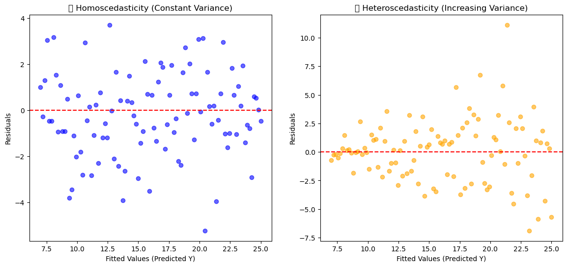
3. Homoscedasticity (Constant Variance of Errors)#
The variance of residuals is the same across all levels of predictors.
In plots: residuals should look like a random “cloud,” not a funnel (widening/narrowing spread).
import numpy as np
import matplotlib.pyplot as plt
import seaborn as sns
import warnings

warnings.filterwarnings('ignore')
# Seed for reproducibility
np.random.seed(42)

# Generate X values
X = np.linspace(1, 10, 100)

# Case 1: Homoscedasticity (constant variance)
y_true = 2 * X + 5
residuals_homo = np.random.normal(0, 2, size=len(X))
y_homo = y_true + residuals_homo

# Case 2: Heteroscedasticity (increasing variance)
residuals_hetero = np.random.normal(0, X/2, size=len(X))  # variance grows with X
y_hetero = y_true + residuals_hetero

# Predictions (fitted values)
y_pred = y_true

# Plotting
fig, axes = plt.subplots(1, 2, figsize=(14, 6))

# Homoscedasticity Plot
axes[0].scatter(y_pred, y_homo - y_pred, color="blue", alpha=0.6)
axes[0].axhline(y=0, color="red", linestyle="--")
axes[0].set_title("✅ Homoscedasticity (Constant Variance)")
axes[0].set_xlabel("Fitted Values (Predicted Y)")
axes[0].set_ylabel("Residuals")

# Heteroscedasticity Plot
axes[1].scatter(y_pred, y_hetero - y_pred, color="orange", alpha=0.6)
axes[1].axhline(y=0, color="red", linestyle="--")
axes[1].set_title("❌ Heteroscedasticity (Increasing Variance)")
axes[1].set_xlabel("Fitted Values (Predicted Y)")
axes[1].set_ylabel("Residuals")

plt.show()
4. Normality of Errors#
Residuals should be normally distributed (especially important for hypothesis testing and confidence intervals).
The line can still fit without this, but statistical inference becomes unreliable.
5. No (or little) Multicollinearity#
Predictors should not be highly correlated with each other.
If they are, coefficients \(\beta\) become unstable and hard to interpret.
Variance Inflation Factor (VIF) is often used to check this.
See the section for details.
6. No Endogeneity (Exogeneity of Predictors)#
Predictors \(X\) should be independent of the error term \(\epsilon\).
If a predictor is correlated with errors, the coefficients are biased.
Classic example: omitted variable bias.
7. Measurement Accuracy#
Predictors should be measured without error.
In practice, small measurement error is tolerable, but large ones distort results.
🔧 Workflow of Regression Models#
Simple Linear Regression#
📌 Relationship between one independent variable (x) and one dependent variable (y).
Workflow:#
Define Model:
\[ y = \beta_0 + \beta_1 x + \epsilon \]Assumptions Check: Linearity, homoscedasticity, independence, normality of residuals.
Cost Function: Minimize MSE:
\[ J(\beta) = \frac{1}{n} \sum (y_i - \hat{y}_i)^2 \]Optimization: Estimate parameters (\(\beta_0, \beta_1\)) using OLS (Ordinary Least Squares) or Gradient Descent.
Train Model: Fit line to data.
Validation: Check residual plots, R², RMSE.
Prediction: Use the line for new \(x\) values.
Multiple Linear Regression#
📌 Relationship between multiple independent variables (x₁, x₂, …, xₚ) and one dependent variable (y).
Workflow:#
Define Model:
\[ y = \beta_0 + \beta_1 x_1 + \beta_2 x_2 + \dots + \beta_p x_p + \epsilon \]Assumptions Check: Same as linear regression + check multicollinearity.
Cost Function:
\[ J(\beta) = \frac{1}{n} \sum (y_i - \hat{y}_i)^2 \]Optimization: Solve for coefficients using matrix form:
\[ \hat{\beta} = (X^TX)^{-1}X^Ty \]Train Model: Fit plane/hyperplane in feature space.
Validation: Use adjusted R², cross-validation, VIF (for multicollinearity).
Prediction: Predict \(y\) given multiple \(x\)’s.
Polynomial Regression#
📌 Extends linear regression by adding polynomial terms (captures non-linear relationships).
Workflow:#
Transform Features: Create polynomial features (e.g., \(x^2, x^3, …\)). Example:
\[ y = \beta_0 + \beta_1 x + \beta_2 x^2 + \beta_3 x^3 + \epsilon \]Assumptions Check: Still linear in coefficients but beware of overfitting.
Cost Function: Same MSE as before.
Optimization: Use OLS or gradient descent to solve for \(\beta\).
Train Model: Fit polynomial curve.
Validation: Use CV to avoid overfitting, check residual plots.
Prediction: Use polynomial curve for predictions.
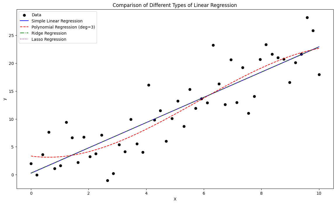
Key Differences in Workflows#
Linear → single predictor, straight line fit.
Multiple Linear → multiple predictors, hyperplane fit.
Polynomial → transformed features, curve fitting (but still linear in parameters).
import matplotlib.pyplot as plt
import numpy as np
from sklearn.linear_model import LinearRegression, Ridge, Lasso
from sklearn.preprocessing import PolynomialFeatures

# Generate synthetic data
np.random.seed(42)
X = np.linspace(0, 10, 50).reshape(-1, 1)
y = 2.5 * X.flatten() + np.random.normal(0, 4, size=50)

# Models
lin_reg = LinearRegression().fit(X, y)
poly = PolynomialFeatures(degree=3)
X_poly = poly.fit_transform(X)
poly_reg = LinearRegression().fit(X_poly, y)

ridge_reg = Ridge(alpha=1.0).fit(X, y)
lasso_reg = Lasso(alpha=0.1).fit(X, y)

# Predictions
x_range = np.linspace(0, 10, 200).reshape(-1, 1)
y_lin = lin_reg.predict(x_range)
y_poly = poly_reg.predict(poly.transform(x_range))
y_ridge = ridge_reg.predict(x_range)
y_lasso = lasso_reg.predict(x_range)

# Plot
plt.figure(figsize=(14, 8))

plt.scatter(X, y, color="black", label="Data")

plt.plot(x_range, y_lin, color="blue", label="Simple Linear Regression")
plt.plot(x_range, y_poly, color="red", linestyle="--", label="Polynomial Regression (deg=3)")
plt.plot(x_range, y_ridge, color="green", linestyle="-.", label="Ridge Regression")
plt.plot(x_range, y_lasso, color="purple", linestyle=":", label="Lasso Regression")

plt.title("Comparison of Different Types of Linear Regression")
plt.xlabel("X")
plt.ylabel("y")
plt.legend()
plt.show()