Hyperparameter Tuning#
Unlike algorithms like Random Forest or SVM, PCA has very few hyperparameters, but the main ones are:
a) Number of components (n_components)#
Definition: The number of principal components to keep (k).
Effect:
Too small → lose too much information (high reconstruction error).
Too large → include noise, less dimensionality reduction benefit.
b) Whiten#
Definition: Whether to scale the principal components to unit variance.
Effect:
whiten=True→ components are decorrelated and scaled.Useful for feeding into algorithms sensitive to scale (like k-NN, SVM).
c) Solver#
Options:
auto,full,arpack,randomizedEffect: Determines algorithm to compute SVD (can affect speed for large datasets).
2. Hyperparameter Tuning Goal#
For PCA, tuning usually means selecting n_components to balance:
Variance explained: Keep enough components to capture most variance.
Dimensionality reduction: Reduce features as much as possible.
3. Techniques for Tuning n_components#
a) Variance Explained Threshold#
Plot cumulative explained variance ratio and pick components that capture e.g., 90–95% of variance.
Formula:
Where \(\lambda_i\) is the i-th eigenvalue.
Rule of Thumb: Keep the smallest number of components that explains ≥90–95% of variance.
b) Cross-Validation (with downstream task)#
If PCA is used before a supervised learning model:
Try different
n_components.Train your model (e.g., logistic regression) on the reduced data.
Evaluate performance (accuracy, F1-score, etc.).
Pick
n_componentsgiving best validation performance.
This is more robust because variance alone doesn’t guarantee optimal performance for predictive tasks.
c) Scree Plot#
Plot eigenvalues (variance per component) vs component index.
Look for “elbow”, where adding more components gives diminishing returns.
4. Quick Summary Table#
Hyperparameter |
Tuning Strategy |
Notes |
|---|---|---|
|
Variance threshold, CV with downstream model, scree plot |
Most important |
|
Try True/False |
Useful if model sensitive to scale |
|
Depends on data size |
Large datasets → |
Intuition
PCA is unsupervised, so tuning is mostly about information retention.
If using PCA as preprocessing, always validate via model performance after dimensionality reduction.
Handle Overfitting/Underfitting#
PCA is an unsupervised dimensionality reduction technique, so overfitting/underfitting is less direct than in supervised learning. However, it still matters when PCA is used as preprocessing for a model:
Overfitting:
Happens if you retain too many principal components, including noise.
The downstream model learns noise instead of signal.
Underfitting:
Happens if you retain too few principal components, losing important information.
The downstream model cannot capture the true patterns in data.
2. How to Handle Overfitting in PCA#
a) Reduce number of components#
Keep only the components that capture the majority of variance (90–95%).
Discard minor components which may contain noise.
b) Use Cross-Validation#
Evaluate model performance with different
n_components.Choose the number of components that optimizes validation performance.
c) Regularization in downstream models#
Even with PCA, the model itself can overfit. Apply regularization (L1/L2) after dimensionality reduction.
3. How to Handle Underfitting in PCA#
a) Increase number of components#
If too little variance is retained, include more principal components.
b) Feature engineering#
PCA reduces dimensions but cannot create new signal. Ensure important features are not discarded before PCA.
c) Use non-linear dimensionality reduction#
Standard PCA is linear. If patterns are non-linear, try Kernel PCA or t-SNE for better representation.
4. Practical Workflow to Avoid Overfitting/Underfitting#
Standardize data → PCA is sensitive to scale.
Compute explained variance ratio → Decide initial
n_components.Cross-validate downstream model with different
n_components.Monitor performance → Look for improvement plateau to avoid overfitting.
Adjust components → Increase if underfitting, decrease if overfitting.
Intuition
Think of PCA as a filter:
Keep enough components to preserve signal → avoid underfitting.
Discard components that capture noise → avoid overfitting.
import numpy as np
import matplotlib.pyplot as plt
from sklearn.decomposition import PCA
from mpl_toolkits.mplot3d import Axes3D

# Generate synthetic 3D data
np.random.seed(42)
n_samples = 100
X = np.random.rand(n_samples, 2) * 10
Z_noise = np.random.randn(n_samples) * 0.2  # small noise in 3rd dimension
X = np.column_stack((X, 0.5*X[:,0] + 0.2*X[:,1] + Z_noise))

# Apply PCA with different components
components = [1, 2, 3]
reconstructions = []

for k in components:
    pca = PCA(n_components=k)
    X_reduced = pca.fit_transform(X)
    X_reconstructed = pca.inverse_transform(X_reduced)
    reconstructions.append(X_reconstructed)

# Plot original and reconstructed data
fig = plt.figure(figsize=(18, 5))

titles = ["Underfitting (1 Component)", "Good Fit (2 Components)", "Overfitting (3 Components)"]

for i in range(3):
    ax = fig.add_subplot(1, 3, i+1, projection='3d')
    ax.scatter(X[:, 0], X[:, 1], X[:, 2], alpha=0.3, label='Original')
    ax.scatter(reconstructions[i][:, 0], reconstructions[i][:, 1], reconstructions[i][:, 2],
               alpha=0.7, label='Reconstructed')
    ax.set_title(titles[i])
    ax.set_xlabel('X')
    ax.set_ylabel('Y')
    ax.set_zlabel('Z')
    ax.view_init(20, 30)
    ax.legend()

plt.show()
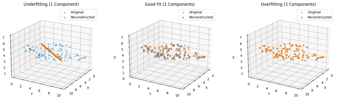
What You’ll See in the 3D Plot#
Underfitting (1 component):
Reconstruction flattens data along a single direction.
Large reconstruction error, main structure lost.
Good Fit (2 components):
Captures main plane of data.
Reconstruction is accurate, minimal loss.
Overfitting (3 components):
Includes tiny noisy 3rd dimension.
Slight improvement in reconstruction but may introduce noise for downstream models.