HyperParameter Tuning#
XGBRegressor#
XGBoost has many knobs, but the most influential ones fall into 3 categories:
Tree complexity (model capacity)#
max_depthMaximum depth of trees.
Large → captures complex patterns but risks overfitting.
Small → prevents overfitting but may underfit.
Typical: 3–10.
min_child_weightMinimum sum of weights (number of samples × sample weight) in a leaf node.
Large → more conservative splits (avoids overfitting).
Small → allows deep trees and complex patterns.
Typical: 1–10.
Boosting process#
n_estimators(a.k.a. boosting rounds)Number of trees added sequentially.
Large → reduces bias, but may overfit if not combined with regularization.
Tune with early stopping.
learning_rate(η)Shrinks each tree’s contribution.
Low η → slower learning, needs more trees but generalizes better.
High η → faster learning, risks overshooting.
Typical: 0.01–0.3.
Sampling (regularization by randomness)#
subsampleFraction of samples used for each tree.
<1.0 introduces randomness → prevents overfitting.
Typical: 0.5–0.9.
colsample_bytree/colsample_bylevel/colsample_bynodeFraction of features sampled at each step.
Lower values → prevent feature dominance & overfitting.
Typical: 0.5–0.9.
Regularization#
reg_lambda(L2 regularization)Penalizes large leaf weights → smoother model.
reg_alpha(L1 regularization)Encourages sparsity (feature selection).
Hyperparameter Tuning Strategy#
Step 1: Start simple#
max_depth=3,learning_rate=0.1,n_estimators=200,subsample=0.8.
Step 2: Tune tree depth & min_child_weight#
Grid search over
max_depth(3–10) andmin_child_weight(1–6).Balance bias (too shallow) vs variance (too deep).
Step 3: Tune gamma (min_split_loss)#
Prevents unnecessary splits.
Try values {0, 0.1, 0.2, …}.
Step 4: Tune subsample & colsample_bytree#
Try ranges {0.5–1.0}.
Introduces randomness to fight overfitting.
Step 5: Tune regularization terms#
Increase
reg_lambdaorreg_alphaif still overfitting.
Step 6: Tune learning rate & n_estimators together#
If overfitting → decrease
learning_rate, increasen_estimators.Use early stopping with a validation set.
3. Handling Overfitting (High Variance)#
👉 Model fits training data too well but fails on unseen data.
Symptoms#
Train error ≪ Test error.
Predictions unstable.
Fixes#
Reduce model complexity:
Lower
max_depth.Increase
min_child_weight.Increase
gamma.
Add randomness:
Lower
subsample,colsample_bytree.
Regularization:
Increase
reg_lambda,reg_alpha.
Learning rate:
Lower
learning_rate, increasen_estimators.
Early stopping:
Stop when validation loss stops improving.
4. Handling Underfitting (High Bias)#
👉 Model is too simple, missing important patterns.
Symptoms#
Both Train & Test error are high.
Predictions too smooth.
Fixes#
Increase model capacity:
Higher
max_depth.Lower
min_child_weight.Reduce
gamma.
Boost longer:
Increase
n_estimators.Or reduce
learning_rateand increasen_estimators.
Use more features:
Increase
colsample_bytree.Ensure dataset has informative features.
Summary:
Overfitting → simplify trees, add regularization, introduce randomness, use early stopping.
Underfitting → deepen trees, reduce regularization, increase estimators, lower learning rate.
Hyperparameter tuning balances bias vs variance → use GridSearchCV / RandomizedSearchCV with cross-validation.
import numpy as np
import matplotlib.pyplot as plt
from sklearn.datasets import make_regression
from sklearn.model_selection import train_test_split, GridSearchCV
from sklearn.metrics import mean_squared_error
from xgboost import XGBRegressor
# -----------------------------
# 1. Synthetic dataset
# -----------------------------
X, y = make_regression(
n_samples=800, n_features=20, noise=25, random_state=42
)
X_train, X_test, y_train, y_test = train_test_split(
X, y, test_size=0.2, random_state=42
)
# -----------------------------
# 2. Function to plot learning curves
# -----------------------------
def plot_learning_curve(model, X_train, y_train, X_test, y_test, label):
eval_set = [(X_train, y_train), (X_test, y_test)]
model.fit(X_train, y_train,
eval_set=eval_set,
verbose=False)
results = model.evals_result()
epochs = len(results['validation_0']['rmse'])
x_axis = range(0, epochs)
plt.plot(x_axis, results['validation_0']['rmse'], label=f'Train - {label}')
plt.plot(x_axis, results['validation_1']['rmse'], label=f'Test - {label}')
# -----------------------------
# 3. Compare underfitting, good fit, overfitting
# -----------------------------
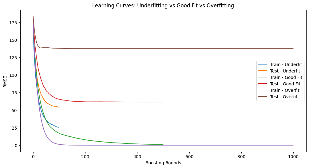
plt.figure(figsize=(12, 6))
# Underfitting model (too simple)
underfit_model = XGBRegressor(
n_estimators=100, max_depth=2, learning_rate=0.3,
subsample=1, colsample_bytree=1, random_state=42
)
plot_learning_curve(underfit_model, X_train, y_train, X_test, y_test, "Underfit")
# Balanced model (good fit)
good_model = XGBRegressor(
n_estimators=500, max_depth=4, learning_rate=0.1,
subsample=0.8, colsample_bytree=0.8, random_state=42
)
plot_learning_curve(good_model, X_train, y_train, X_test, y_test, "Good Fit")
# Overfitting model (too complex, no regularization)
overfit_model = XGBRegressor(
n_estimators=1000, max_depth=10, learning_rate=0.05,
subsample=1, colsample_bytree=1, reg_lambda=0, random_state=42
)
plot_learning_curve(overfit_model, X_train, y_train, X_test, y_test, "Overfit")
plt.xlabel("Boosting Rounds")
plt.ylabel("RMSE")
plt.title("Learning Curves: Underfitting vs Good Fit vs Overfitting")
plt.legend()
plt.show()
# -----------------------------
# 4. Hyperparameter tuning with GridSearchCV
# -----------------------------
param_grid = {
"max_depth": [3, 5, 7],
"min_child_weight": [1, 3, 5],
"gamma": [0, 0.1, 0.3],
"reg_lambda": [0.1, 1, 10]
}
grid = GridSearchCV(
XGBRegressor(
learning_rate=0.1, n_estimators=500,
subsample=0.8, colsample_bytree=0.8,
random_state=42
),
param_grid,
cv=3,
scoring="neg_mean_squared_error",
n_jobs=-1,
verbose=1
)
grid.fit(X_train, y_train)
print("Best Parameters:", grid.best_params_)
print("Best CV Score (MSE):", -grid.best_score_)
# Evaluate best model on test set
best_model = grid.best_estimator_
y_pred = best_model.predict(X_test)
print("Test MSE:", mean_squared_error(y_test, y_pred))
Fitting 3 folds for each of 81 candidates, totalling 243 fits
Best Parameters: {'gamma': 0.3, 'max_depth': 3, 'min_child_weight': 5, 'reg_lambda': 1}
Best CV Score (MSE): 3724.4582271880595
Test MSE: 2760.9442892671045
XGBClassifier#
XGBoost has many knobs to tune. They fall into 4 broad categories:
1. Tree complexity (model capacity)#
These control bias vs variance (underfitting vs overfitting).
max_depth: Maximum depth of each tree.Too small → high bias (underfit).
Too large → high variance (overfit).
min_child_weight: Minimum sum of instance weights (hessian) needed in a child node.Larger → more conservative splits (prevents overfitting).
gamma: Minimum loss reduction required to make a split.Larger → fewer splits (more conservative).
2. Sampling techniques (regularization via randomness)#
These help reduce variance and prevent overfitting.
subsample: Fraction of rows sampled for each tree.Lower → reduces variance (like bagging).
colsample_bytree/colsample_bylevel: Fraction of features sampled.Prevents reliance on a few strong features.
3. Regularization parameters (explicit penalties)#
reg_lambda(L2 penalty): Shrinks weights (default = 1). Helps prevent overfitting.reg_alpha(L1 penalty): Drives some weights to zero (feature selection effect).
4. Boosting process (learning dynamics)#
learning_rate (eta): Step size shrinkage.Small → requires more trees but generalizes better.
n_estimators: Number of trees (boosting rounds).Too high without regularization → overfit.
scale_pos_weight: For handling imbalanced classes.
Handling Underfitting & Overfitting#
Underfitting (model too simple)#
Symptoms:
Both training and test accuracy are low.
Training loss is high.
Fix:
Increase
max_depthor decreasemin_child_weight.Decrease
gamma(allow more splits).Increase
n_estimators.Lower regularization (
reg_lambda,reg_alpha).Increase learning rate (to learn faster).
Overfitting (model too complex)#
Symptoms:
Training accuracy is very high, but test accuracy is low.
Training loss keeps decreasing but validation loss increases.
Fix:
Reduce
max_depth.Increase
min_child_weight(more conservative splits).Increase
gamma.Use smaller
learning_ratewith largern_estimators.Use subsampling (
subsample < 1,colsample_bytree < 1).Increase regularization (
reg_lambda,reg_alpha).Use early stopping (
early_stopping_rounds).
🔹 Hyperparameter Tuning Strategy#
Start with learning rate and n_estimators
Choose a small learning rate (0.05–0.1).
Increase
n_estimatorsaccordingly.
Tune tree depth & min_child_weight
Grid search typical values:
max_depth = [3,5,7],min_child_weight = [1,3,5].
Tune gamma
Try
gamma = [0, 0.1, 0.3, 0.5].
Tune subsample & colsample_bytree
Try
[0.6, 0.8, 1.0].
Add regularization
Adjust
reg_lambdaandreg_alpha.
Use cross-validation + early stopping
Prevents overfitting while tuning.
🔹 Example in Practice#
from xgboost import XGBClassifier
from sklearn.datasets import make_classification
from sklearn.model_selection import train_test_split, GridSearchCV
from sklearn.metrics import accuracy_score
import warnings
warnings.filterwarnings("ignore")
# Dataset
X, y = make_classification(n_samples=1000, n_features=20, random_state=42)
X_train, X_test, y_train, y_test = train_test_split(X, y, test_size=0.2, random_state=42)

# Base model
model = XGBClassifier(use_label_encoder=False, eval_metric="logloss")

# Hyperparameter grid
param_grid = {
    "max_depth": [3, 5, 7],
    "min_child_weight": [1, 3, 5],
    "gamma": [0, 0.2, 0.4],
    "subsample": [0.8, 1.0],
    "colsample_bytree": [0.8, 1.0],
    "reg_lambda": [1, 5, 10]
}

# Grid Search
grid = GridSearchCV(model, param_grid, scoring="accuracy", cv=3, verbose=1, n_jobs=-1)
grid.fit(X_train, y_train)

print("Best Parameters:", grid.best_params_)
best_model = grid.best_estimator_

# Evaluate
y_pred = best_model.predict(X_test)
print("Test Accuracy:", accuracy_score(y_test, y_pred))
Fitting 3 folds for each of 324 candidates, totalling 972 fits
Best Parameters: {'colsample_bytree': 1.0, 'gamma': 0.4, 'max_depth': 5, 'min_child_weight': 1, 'reg_lambda': 10, 'subsample': 1.0}
Test Accuracy: 0.895