Performance Metrics#
1. Internal Metrics (No Ground Truth Needed)#
These metrics evaluate how well the clustering captures cohesion and separation.
a) Silhouette Score#
Measures how similar a point is to its own cluster vs other clusters.
Formula for point \(i\):
where:
\(a(i)\) = average distance from \(i\) to points in its own cluster
\(b(i)\) = minimum average distance from \(i\) to points in other clusters
Interpretation:
\(s(i) \approx 1\) → well-clustered
\(s(i) \approx 0\) → on boundary
\(s(i) < 0\) → likely misclustered
b) Davies-Bouldin Index (DBI)#
Measures average similarity between each cluster and its most similar cluster.
\(\sigma_i\) = average distance of points in cluster \(i\) to its centroid
\(d_{ij}\) = distance between cluster centroids \(i\) and \(j\)
Interpretation:
Lower DBI → better clustering (more separation, less overlap)
c) Calinski-Harabasz Index (CH)#
Ratio of between-cluster dispersion to within-cluster dispersion:
Higher CH → better defined clusters
d) Cophenetic Correlation Coefficient (CCC)#
Measures how well the dendrogram preserves original pairwise distances:
\(d_{ij}\) = original distance between points \(i\) and \(j\)
\(d_{ij}^{\text{dendrogram}}\) = height at which \(i\) and \(j\) merge in dendrogram
Interpretation:
CCC close to 1 → dendrogram preserves pairwise distances well
Useful for validating hierarchical structure
2. External Metrics (Ground Truth Available)#
If true labels are known (rare in real-world unsupervised tasks), we can use:
a) Adjusted Rand Index (ARI)#
Measures agreement between predicted clusters and true labels, adjusted for chance
ARI = 1 → perfect match, ARI ≈ 0 → random
b) Normalized Mutual Information (NMI)#
Measures shared information between predicted clusters and true labels
NMI = 1 → perfect match, NMI = 0 → no mutual information
c) Fowlkes-Mallows Index (FMI)#
Geometric mean of precision and recall between predicted clusters and true labels
Range: 0–1, higher is better
3. Practical Notes#
Choose internal metrics for real unsupervised tasks, since true labels are usually unknown.
Cophenetic correlation coefficient is especially useful for hierarchical clustering, because it measures how well the dendrogram represents distances.
Silhouette and Davies-Bouldin can help decide optimal number of clusters by cutting the dendrogram at different heights.
Summary Table
Metric |
Type |
Goal |
Higher/Lower Better |
|---|---|---|---|
Silhouette Score |
Internal |
Cohesion vs separation |
Higher |
Davies-Bouldin Index |
Internal |
Cluster similarity |
Lower |
Calinski-Harabasz Index |
Internal |
Between/within dispersion |
Higher |
Cophenetic Correlation |
Internal |
Dendrogram quality |
Higher |
Adjusted Rand Index |
External |
Match with true labels |
Higher |
Normalized Mutual Info |
External |
Shared info with labels |
Higher |
Fowlkes-Mallows |
External |
Precision/recall |
Higher |
import numpy as np
import matplotlib.pyplot as plt
from sklearn.datasets import make_blobs
from sklearn.preprocessing import StandardScaler
from sklearn.metrics import silhouette_score, davies_bouldin_score, calinski_harabasz_score
from scipy.cluster.hierarchy import linkage, fcluster, cophenet
from scipy.spatial.distance import pdist
# Step 1: Generate synthetic dataset
X, y_true = make_blobs(n_samples=100, centers=3, n_features=2, random_state=42)
X = StandardScaler().fit_transform(X)
# Step 2: Compute linkage matrix using Ward's method
Z = linkage(X, method='ward')
# Step 3: Evaluate dendrogram with different numbers of clusters
num_clusters = [2, 3, 4, 5]
metrics_results = []
for k in num_clusters:
labels = fcluster(Z, t=k, criterion='maxclust')
silhouette = silhouette_score(X, labels)
dbi = davies_bouldin_score(X, labels)
ch = calinski_harabasz_score(X, labels)
ccc, _ = cophenet(Z, pdist(X))
metrics_results.append((k, silhouette, dbi, ch, ccc))
# Step 4: Display results
print("Clusters | Silhouette | Davies-Bouldin | Calinski-Harabasz | Cophenetic Corr")
for row in metrics_results:
print(f"{row[0]:>7} | {row[1]:>10.3f} | {row[2]:>14.3f} | {row[3]:>16.3f} | {row[4]:>15.3f}")
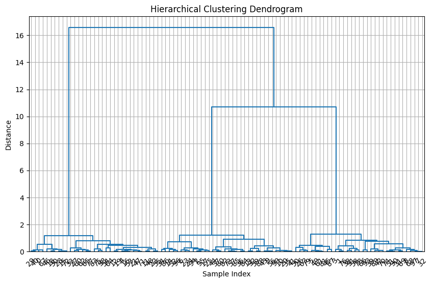
# Step 5: Plot dendrogram
plt.figure(figsize=(10, 6))
from scipy.cluster.hierarchy import dendrogram
dendrogram(Z, color_threshold=0, leaf_rotation=45, leaf_font_size=10)
plt.title("Hierarchical Clustering Dendrogram")
plt.xlabel("Sample Index")
plt.ylabel("Distance")
plt.grid(True)
plt.show()
Clusters | Silhouette | Davies-Bouldin | Calinski-Harabasz | Cophenetic Corr
      2 |      0.687 |          0.459 |          214.067 |           0.977
      3 |      0.849 |          0.210 |         1686.708 |           0.977
      4 |      0.679 |          0.574 |         1308.390 |           0.977
      5 |      0.518 |          0.854 |         1146.523 |           0.977