Lasso Regression#
Lasso stands for Least Absolute Shrinkage and Selection Operator. It’s a linear regression technique that uses L1 regularization to:
Reduce overfitting.
Perform feature selection by shrinking some coefficients to exactly zero.
The L1 Regularization Formula#
In ordinary least squares (OLS), we minimize:
In Lasso, we add a penalty term:
Where:
\(\lambda\) = regularization parameter (controls penalty strength).
\(|\beta_j|\) = absolute value of coefficient.
Intercept (\(\beta_0\)) is usually not penalized.
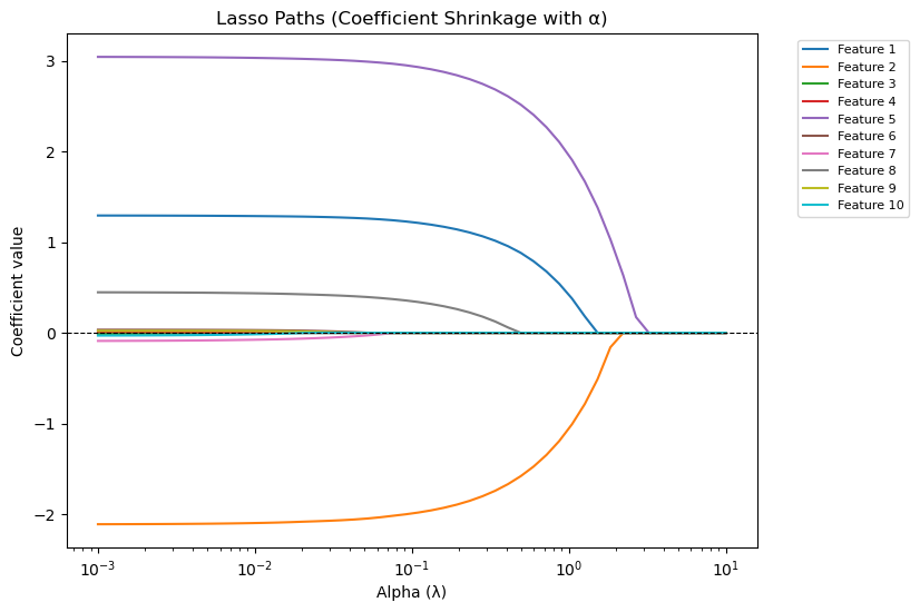
Effect of L1 Penalty#
If λ = 0 → Same as OLS (no regularization).
If λ is small → Slight shrinkage, coefficients reduced but most remain non-zero.
If λ is large → Many coefficients shrink to exactly zero (feature elimination).
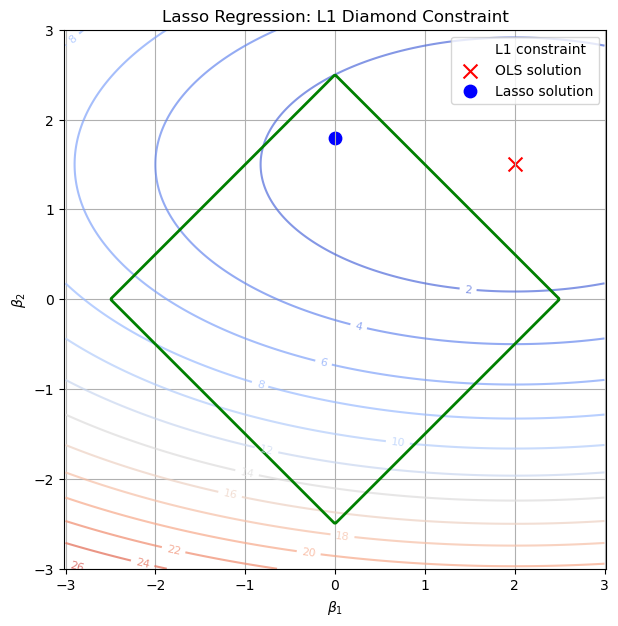
Why Lasso Can Zero Out Coefficients#
Mathematically, the absolute value function creates sharp corners in the cost function’s geometry (diamond-shaped constraint), so the optimization often hits exactly zero for some coefficients. This is different from Ridge (L2), which only shrinks coefficients but never makes them exactly zero.
When to Use Lasso#
✅ When you suspect many irrelevant features. ✅ When you want automatic feature selection. ✅ When you have high-dimensional data (p >> n).
Visual Intuition#
Think of it as forcing coefficients to live inside a diamond-shaped boundary.
Because of the diamond’s corners, optimization naturally “sticks” some coefficients at zero.
import numpy as np
import matplotlib.pyplot as plt
import warnings

warnings.filterwarnings("ignore")
# Create grid of coefficients
beta1 = np.linspace(-3, 3, 400)
beta2 = np.linspace(-3, 3, 400)
B1, B2 = np.meshgrid(beta1, beta2)

# Lasso constraint (diamond): |beta1| + |beta2| <= t
lasso_constraint = np.abs(B1) + np.abs(B2)

# Example OLS solution (unregularized minimum)
ols_point = np.array([2.0, 1.5])

# Simulated contour of RSS (elliptical error surface)
rss = (B1 - ols_point[0])**2/4 + (B2 - ols_point[1])**2

plt.figure(figsize=(7,7))

# RSS contours
cs = plt.contour(B1, B2, rss, levels=15, cmap="coolwarm", alpha=0.7)
plt.clabel(cs, inline=1, fontsize=8)

diamond_boundary = plt.contour(
    B1, B2, lasso_constraint,
    levels=[2.5],
    colors="green",
    linewidths=2,
    label="L1 constraint"
)


# Lasso constraint region (diamond)
# diamond_boundary = plt.contour(B1, B2, lasso_constraint, levels=[2.5], colors="green", linewidths=2)
# diamond_boundary.collections[0].set_label("L1 constraint")

# Mark OLS solution
plt.scatter(*ols_point, color="red", marker="x", s=100, label="OLS solution")

# Approx Lasso solution (where ellipse first touches diamond corner)
lasso_point = np.array([0, 1.8])  # coefficient on β1 shrinks to zero
plt.scatter(*lasso_point, color="blue", marker="o", s=80, label="Lasso solution")

plt.xlabel(r"$\beta_1$")
plt.ylabel(r"$\beta_2$")
plt.title("Lasso Regression: L1 Diamond Constraint")
plt.legend()
plt.grid(True)
plt.axis("equal")
plt.show()
The Kernel crashed while executing code in the current cell or a previous cell.

Please review the code in the cell(s) to identify a possible cause of the failure.

Click <a href='https://aka.ms/vscodeJupyterKernelCrash'>here</a> for more info.

View Jupyter <a href='command:jupyter.viewOutput'>log</a> for further details.
import numpy as np
import matplotlib.pyplot as plt
from sklearn.linear_model import Lasso
from sklearn.preprocessing import StandardScaler

# Generate synthetic dataset
np.random.seed(42)
X = np.random.randn(100, 10)
y = X @ np.array([1.5, -2, 0, 0, 3, 0, 0, 0.5, 0, 0]) + np.random.randn(100) * 0.5

# Standardize features
scaler = StandardScaler()
X_scaled = scaler.fit_transform(X)

# Range of alpha values
alphas = np.logspace(-3, 1, 50)
coefs = []

# Fit Lasso for each alpha
for a in alphas:
    lasso = Lasso(alpha=a, max_iter=10000)
    lasso.fit(X_scaled, y)
    coefs.append(lasso.coef_)

coefs = np.array(coefs)

# Plot coefficient paths
plt.figure(figsize=(8, 6))
for i in range(coefs.shape[1]):
    plt.plot(alphas, coefs[:, i], label=f"Feature {i+1}")

plt.xscale("log")
plt.xlabel("Alpha (λ)")
plt.ylabel("Coefficient value")
plt.title("Lasso Paths (Coefficient Shrinkage with α)")
plt.axhline(0, color="black", linestyle="--", linewidth=0.8)
plt.legend(bbox_to_anchor=(1.05, 1), loc="upper left", fontsize=8)
plt.show()