Ensembling#
Ensembling is the process of combining multiple models (often called weak learners) to create a stronger overall model.
Goal: Improve predictive performance and reduce errors.
Motivation: A single model may make mistakes due to bias or variance. By combining models, we average out errors.
2. Why Ensembling Works#
Different models make different errors.
If errors are uncorrelated, averaging or voting can cancel them out.
Leads to better generalization on unseen data.
Example (Intuition):
Suppose 3 models predict the price of a house:
Model A → 100k
Model B → 120k
Model C → 110k
Ensemble (average) → 110k → closer to actual value than any single model.
3. Types of Ensembling#
There are two main types: Bagging and Boosting.
A. Bagging (Bootstrap Aggregating)#
Idea: Train multiple models independently on different random subsets of data, then combine predictions.
Steps:
Sample dataset with replacement (bootstrap) to create multiple subsets.
Train a model on each subset (e.g., Decision Tree).
Aggregate predictions:
Regression → average
Classification → majority vote
Characteristics:
Reduces variance
Prevents overfitting of a single model
Example: Random Forest
Each tree sees a different subset of data and features.
Predictions are averaged → smoother, more stable.
B. Boosting#
Idea: Train models sequentially, each learning from the errors of the previous model.
Steps:
Train the first weak learner.
Identify the mistakes it made.
Train the next learner to focus more on the mistakes.
Repeat and combine all learners into a weighted sum.
Characteristics:
Reduces bias
Can overfit if too many learners or learning rate too high
Popular Boosting Algorithms:
AdaBoost
Gradient Boosting
XGBoost, LightGBM, CatBoost
C. Stacking (Stacked Generalization)#
Idea: Combine predictions of multiple models using a meta-model.
Steps:
Train multiple base models on the dataset.
Use their predictions as features to train a meta-model.
Meta-model learns how to best combine the base models.
Characteristics:
Can leverage diverse model types
Often improves accuracy beyond Bagging or Boosting
4. Benefits of Ensembling#
Better accuracy and stability
Reduces variance and/or bias
Makes models more robust to noise and outliers
5. Trade-offs / Limitations#
Complexity: Harder to interpret than a single model
Training time: Can be much slower (many models instead of one)
Memory usage: Stores multiple models
Summary Table#
Type |
How it Works |
Reduces |
Example |
|---|---|---|---|
Bagging |
Train on random subsets independently |
Variance |
Random Forest |
Boosting |
Train sequentially, focus on errors |
Bias |
AdaBoost, GradientBoost |
Stacking |
Combine predictions using meta-model |
Bias + Variance |
Stacked models |
Ensembling is basically “strength in numbers” — multiple weak models together usually perform much better than one alone.
# Step 1: Import Libraries
import numpy as np
import matplotlib.pyplot as plt
from sklearn.model_selection import train_test_split
from sklearn.tree import DecisionTreeRegressor
from sklearn.ensemble import RandomForestRegressor, GradientBoostingRegressor
from sklearn.metrics import mean_squared_error, r2_score
# Step 2: Create Sample Dataset
np.random.seed(42)
X = np.sort(np.random.rand(100, 1) * 10, axis=0)
y = np.sin(X).ravel() + np.random.normal(0, 0.3, X.shape[0])
X_train, X_test, y_train, y_test = train_test_split(X, y, test_size=0.3, random_state=42)
# Step 3: Initialize Models
dt = DecisionTreeRegressor(max_depth=None, random_state=42)
rf = RandomForestRegressor(n_estimators=100, max_depth=None, random_state=42)
gbr = GradientBoostingRegressor(n_estimators=100, learning_rate=0.1, max_depth=3, random_state=42)
# Step 4: Train Models
dt.fit(X_train, y_train)
rf.fit(X_train, y_train)
gbr.fit(X_train, y_train)
# Step 5: Predictions
X_plot = np.linspace(0, 10, 200).reshape(-1, 1)
y_dt = dt.predict(X_plot)
y_rf = rf.predict(X_plot)
y_gbr = gbr.predict(X_plot)
# Step 6: Metrics
def print_metrics(name, y_true, y_pred):
print(f"{name}: R²={r2_score(y_true, y_pred):.2f}, RMSE={np.sqrt(mean_squared_error(y_true, y_pred)):.2f}")
print_metrics("Decision Tree", y_test, dt.predict(X_test))
print_metrics("Random Forest (Bagging)", y_test, rf.predict(X_test))
print_metrics("Gradient Boosting (Boosting)", y_test, gbr.predict(X_test))
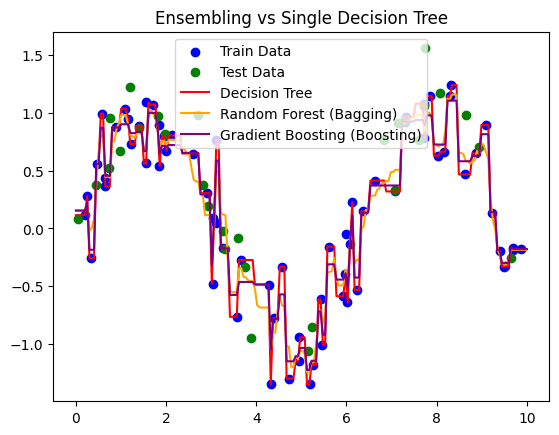
# Step 7: Plot Predictions
plt.scatter(X_train, y_train, color='blue', label='Train Data')
plt.scatter(X_test, y_test, color='green', label='Test Data')
plt.plot(X_plot, y_dt, color='red', label='Decision Tree')
plt.plot(X_plot, y_rf, color='orange', label='Random Forest (Bagging)')
plt.plot(X_plot, y_gbr, color='purple', label='Gradient Boosting (Boosting)')
plt.legend()
plt.title("Ensembling vs Single Decision Tree")
plt.show()
Decision Tree: R²=0.71, RMSE=0.35
Random Forest (Bagging): R²=0.78, RMSE=0.31
Gradient Boosting (Boosting): R²=0.80, RMSE=0.29