Cost Functions#
A cost function measures how well a regression line fits the data. It calculates the error (difference between predicted and actual values). The goal is to find parameters (\(\theta_0, \theta_1, ...\)) that minimize this cost.
Mean Squared Error (MSE)#
Most common cost function for linear regression.
Squares the errors → penalizes large errors heavily.
Smooth and differentiable → great for gradient descent.
✅ Pros:
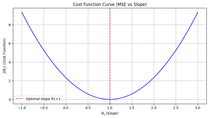
Convex function → guarantees global minimum.
Emphasizes large errors (good for minimizing outliers’ impact in general trend fitting).
❌ Cons:
Sensitive to outliers → a single extreme point can distort results.
Mean Absolute Error (MAE)#
Takes absolute differences instead of squaring.
Errors are treated equally (linear penalty).
✅ Pros:
Robust to outliers (doesn’t blow up error).
Simple interpretation (average error in same units as data).
❌ Cons:
Not differentiable at zero (gradient descent is trickier, though solvable with subgradients).
Optimization can be slower.
Huber Loss (Combination of MSE and MAE)#
Uses MSE for small errors (smooth) and MAE for large errors (robust to outliers).
✅ Pros:
Best of both worlds: smooth optimization + outlier resistance.
Widely used in robust regression.
❌ Cons:
Need to choose hyperparameter \(\delta\).
Log-Cosh Loss#
Behaves like MSE for small errors and like MAE for large errors (but smoother).
✅ Pros:
Smooth everywhere (better for gradient descent).
Less sensitive to outliers than MSE.
❌ Cons:
Computationally more expensive than MSE.
Quantile Loss (Pinball Loss)#
Used in quantile regression (instead of predicting mean, predicts quantiles like median, 90th percentile).
For \(q=0.5\), it reduces to MAE (median regression).
✅ Pros:
Useful for risk-sensitive domains (finance, forecasting).
❌ Cons:
More complex interpretation.
Impact of Cost Functions#
MSE → great for general regression, but heavily penalizes outliers.
MAE → robust to outliers but optimization harder.
Huber / Log-Cosh → balance between robustness and efficiency.
Quantile Loss → gives flexibility beyond “average prediction”.
👉 In standard linear regression, we almost always use MSE because:
It’s mathematically elegant (derivative gives closed-form solution).
Convex → guarantees global minimum.
Easy to optimize with gradient descent or normal equation.
import numpy as np
import matplotlib.pyplot as plt

# Sample dataset (simple linear data)
X = np.array([1, 2, 3])
y = np.array([1, 2, 3])
m = len(y)

# Hypothesis function h(x) = theta1 * x (assuming theta0 = 0 for simplicity)
def hypothesis(theta1, X):
    return theta1 * X

# Cost function J(theta1)
def cost(theta1, X, y):
    return (1/(2*m)) * np.sum((hypothesis(theta1, X) - y) ** 2)

# Generate values of theta1 to test
theta1_vals = np.linspace(-1, 3, 100)
J_vals = [cost(t, X, y) for t in theta1_vals]

# Plot the cost function curve
plt.figure(figsize=(10,5))
plt.plot(theta1_vals, J_vals, color='blue')
plt.xlabel(r"$\theta_1$ (Slope)")
plt.ylabel(r"$J(\theta_1)$ (Cost Function)")
plt.title("Cost Function Curve (MSE vs Slope)")
plt.axvline(x=1, color='red', linestyle="--", label="Optimal slope θ1=1")
plt.legend()
plt.grid(True)
plt.show()