Hyperparameter Tuning#
Gradient Boosting Regressor#
Hyperparameters control model complexity, learning speed, and generalization. Key ones:
Hyperparameter |
Role / Effect |
|---|---|
|
Number of weak learners (trees). Too high → overfitting; too low → underfitting. |
|
Shrinkage factor applied to each tree. Smaller → slower learning, reduces overfitting. |
|
Maximum depth of each tree. Higher depth → more complex trees → risk of overfitting. |
|
Minimum samples required to split a node. Higher → simpler trees → prevents overfitting. |
|
Minimum samples required at a leaf. Higher → prevents overfitting. |
|
Fraction of data used for each tree (stochastic gradient boosting). Reduces variance. |
|
Max features considered at each split. Reduces correlation between trees, reduces overfitting. |
|
Loss function (MSE, MAE, Huber). Controls sensitivity to outliers. |
Hyperparameter Tuning Strategies#
Grid Search
from sklearn.model_selection import GridSearchCV
from sklearn.ensemble import GradientBoostingRegressor

param_grid = {
    'n_estimators': [50, 100, 200],
    'learning_rate': [0.01, 0.05, 0.1],
    'max_depth': [2, 3, 4],
    'subsample': [0.8, 1.0]
}

gbr = GradientBoostingRegressor()
grid_search = GridSearchCV(gbr, param_grid, cv=5, scoring='neg_mean_squared_error')
grid_search.fit(X_train, y_train)
best_params = grid_search.best_params_
Randomized Search – faster for large grids, samples combinations randomly.
Early Stopping – monitor validation error to stop adding trees automatically:
gbr = GradientBoostingRegressor(n_estimators=1000, validation_fraction=0.1,
                                n_iter_no_change=10, tol=1e-4)
gbr.fit(X_train, y_train)
3. Handling Overfitting#
Signs: training error is much lower than validation error.
Strategies:
Reduce
n_estimatorsormax_depth.Increase
min_samples_split/min_samples_leaf.Reduce
learning_rateand increasen_estimators(slower, smoother learning).Use
subsample < 1.0(stochastic gradient boosting).Limit
max_featuresto reduce tree correlation.Use early stopping with validation set.
4. Handling Underfitting#
Signs: both training and validation errors are high.
Strategies:
Increase
n_estimators(more trees).Increase
max_depth(more complex trees).Reduce
min_samples_split/min_samples_leaf(allows finer splits).Increase
learning_rateto allow faster learning.Ensure sufficient features in
max_features.
5. Workflow for Tuning GBR#
Start with shallow trees (
max_depth=2-3) and smalllearning_rate=0.05-0.1.Increase
n_estimatorsgradually, monitor validation error.If overfitting occurs → reduce depth, increase
min_samples_leaf, decreaselearning_rate, or usesubsample.If underfitting → increase depth, increase
learning_rate, increasen_estimators.Use cross-validation for robust parameter selection.
Key Intuition
Learning rate vs n_estimators: smaller learning rate + more trees → smoother learning, lower risk of overfitting.
Tree complexity: deeper trees → fit training data closely → risk of overfitting.
Stochastic subsampling: reduces variance, improves generalization.
Demonstration#
import numpy as np
import matplotlib.pyplot as plt
from sklearn.ensemble import GradientBoostingRegressor
# -------------------------------
# Create a synthetic dataset
# -------------------------------
np.random.seed(0)
X = np.linspace(0, 10, 50).reshape(-1,1)
y = np.sin(X).ravel() + np.random.normal(0, 0.2, X.shape[0]) # noisy sine wave
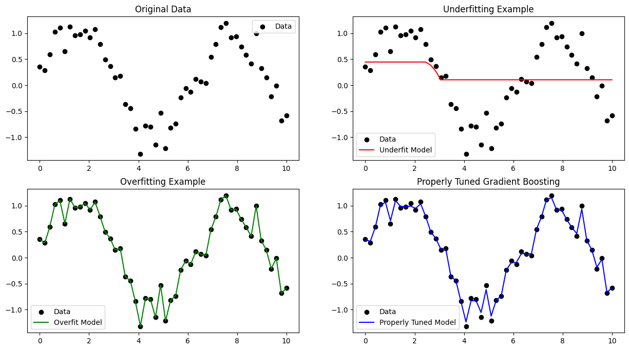
plt.figure(figsize=(15,8))
plt.subplot(2,2,1)
plt.scatter(X, y, color='black', label='Data')
plt.title("Original Data")
plt.legend()
# -------------------------------
# Underfitting example
# -------------------------------
gbr_under = GradientBoostingRegressor(n_estimators=10, max_depth=1, learning_rate=0.05)
gbr_under.fit(X, y)
y_pred_under = gbr_under.predict(X)
plt.subplot(2,2,2)
plt.scatter(X, y, color='black', label='Data')
plt.plot(X, y_pred_under, color='red', label='Underfit Model')
plt.title("Underfitting Example")
plt.legend()
# -------------------------------
# Overfitting example
# -------------------------------
gbr_over = GradientBoostingRegressor(n_estimators=500, max_depth=5, learning_rate=0.2)
gbr_over.fit(X, y)
y_pred_over = gbr_over.predict(X)
plt.subplot(2,2,3)
plt.scatter(X, y, color='black', label='Data')
plt.plot(X, y_pred_over, color='green', label='Overfit Model')
plt.title("Overfitting Example")
plt.legend()
# -------------------------------
# Properly tuned example
# -------------------------------
gbr_tuned = GradientBoostingRegressor(n_estimators=100, max_depth=3, learning_rate=0.1)
gbr_tuned.fit(X, y)
y_pred_tuned = gbr_tuned.predict(X)
plt.subplot(2,2,4)
plt.scatter(X, y, color='black', label='Data')
plt.plot(X, y_pred_tuned, color='blue', label='Properly Tuned Model')
plt.title("Properly Tuned Gradient Boosting")
plt.legend()
plt.show()
Interpretation#
Underfitting (
n_estimators=10,max_depth=1,learning_rate=0.05)Model is too simple → cannot capture sine wave pattern.
Both training and test errors are high.
Overfitting (
n_estimators=500,max_depth=5,learning_rate=0.2)Model is too complex → fits noise in training data.
Low training error, high validation error.
Properly tuned (
n_estimators=100,max_depth=3,learning_rate=0.1)Balanced complexity → captures main pattern without fitting noise.
Best generalization.
Gradient Boosting Classifier#
Here’s a detailed explanation for Gradient Boosting Classifier (GBC) regarding hyperparameter tuning, overfitting, and underfitting:
Hyperparameter |
Role / Effect |
|---|---|
|
Number of weak learners (trees). Too high → overfitting; too low → underfitting. |
|
Shrinkage factor applied to each tree. Smaller → slower learning, reduces overfitting. |
|
Maximum depth of each tree. Higher depth → more complex trees → risk of overfitting. |
|
Minimum samples required to split a node. Higher → simpler trees → prevents overfitting. |
|
Minimum samples required at a leaf. Higher → prevents overfitting. |
|
Fraction of data used for each tree (stochastic gradient boosting). Reduces variance. |
|
Max features considered at each split. Reduces correlation between trees, reduces overfitting. |
|
Loss function ( |
2. Hyperparameter Tuning Strategies#
Grid Search
from sklearn.model_selection import GridSearchCV
from sklearn.ensemble import GradientBoostingClassifier

param_grid = {
    'n_estimators': [50, 100, 200],
    'learning_rate': [0.01, 0.05, 0.1],
    'max_depth': [2, 3, 4],
    'subsample': [0.8, 1.0]
}

gbc = GradientBoostingClassifier()
grid_search = GridSearchCV(gbc, param_grid, cv=5, scoring='accuracy')
grid_search.fit(X_train, y_train)
best_params = grid_search.best_params_
Randomized Search – faster for large grids, samples combinations randomly.
Early Stopping – stop adding trees when validation accuracy stops improving:
gbc = GradientBoostingClassifier(n_estimators=1000, validation_fraction=0.1,
                                 n_iter_no_change=10, tol=1e-4)
gbc.fit(X_train, y_train)
3. Handling Overfitting#
Signs: training accuracy is high, validation accuracy is low.
Strategies:
Reduce
max_depthorn_estimators.Reduce
learning_rateand increasen_estimators.Increase
min_samples_splitormin_samples_leaf.Use
subsample < 1.0to train each tree on a subset.Limit
max_featuresto reduce correlation between trees.Use early stopping on a validation set.
4. Handling Underfitting#
Signs: both training and validation accuracy are low.
Strategies:
Increase
n_estimatorsto allow more boosting rounds.Increase
max_depthfor more complex trees.Decrease
min_samples_split/min_samples_leafto allow finer splits.Increase
learning_ratefor faster learning.Include more features by adjusting
max_features.
5. Workflow for Tuning GBC#
Start with shallow trees (
max_depth=2-3) and smalllearning_rate=0.05-0.1.Gradually increase
n_estimators, monitoring validation accuracy.If overfitting → reduce depth, increase
min_samples_leaf, decreaselearning_rate, usesubsample < 1.If underfitting → increase depth, increase
learning_rate, increasen_estimators.Cross-validation is essential for robust hyperparameter selection.
Key Intuition
Learning rate vs n_estimators: smaller learning rate + more trees → slower but smoother learning, reduces overfitting.
Tree complexity: deeper trees → fit training data closely → risk of overfitting.
Subsampling: reduces variance, improves generalization.
Demonstration#
import numpy as np
import matplotlib.pyplot as plt
from sklearn.ensemble import GradientBoostingClassifier
from sklearn.datasets import make_classification
from matplotlib.colors import ListedColormap
import warnings
warnings.filterwarnings("ignore")
# -------------------------------
# Create a synthetic binary dataset
# -------------------------------
X, y = make_classification(n_samples=200, n_features=2, n_informative=2,
n_redundant=0, n_clusters_per_class=1, random_state=0)
plt.figure(figsize=(15,8))
# Function to plot decision boundary
def plot_decision_boundary(model, X, y, title,axis=(1,1,1)):
cmap_light = ListedColormap(['#FFAAAA', '#AAFFAA'])
cmap_bold = ListedColormap(['#FF0000', '#00FF00'])
x_min, x_max = X[:, 0].min() - 1, X[:,0].max() + 1
y_min, y_max = X[:,1].min() - 1, X[:,1].max() + 1
xx, yy = np.meshgrid(np.arange(x_min, x_max, 0.05),
np.arange(y_min, y_max, 0.05))
Z = model.predict(np.c_[xx.ravel(), yy.ravel()])
Z = Z.reshape(xx.shape)
plt.subplot(*axis)
plt.contourf(xx, yy, Z, cmap=cmap_light, alpha=0.4)
plt.scatter(X[:,0], X[:,1], c=y, cmap=cmap_bold, edgecolor='k')
plt.title(title)
plt.legend()
# -------------------------------
# Underfitting example
# -------------------------------
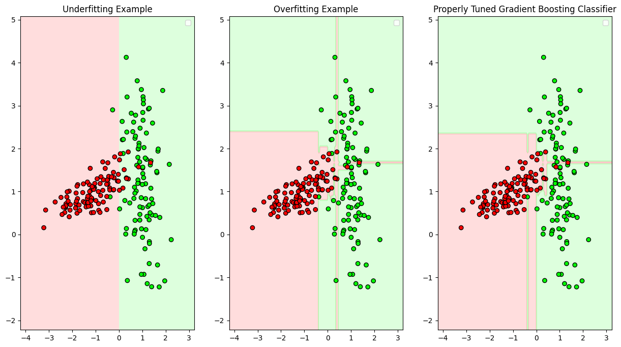
gbc_under = GradientBoostingClassifier(n_estimators=10, max_depth=1, learning_rate=0.05)
gbc_under.fit(X, y)
# plt.subplot(1,3,1)
plot_decision_boundary(gbc_under, X, y, "Underfitting Example",axis=(1,3,1))
# -------------------------------
# Overfitting example
# -------------------------------
gbc_over = GradientBoostingClassifier(n_estimators=500, max_depth=5, learning_rate=0.2)
gbc_over.fit(X, y)
# plt.subplot(1,3,2)
plot_decision_boundary(gbc_over, X, y, "Overfitting Example",axis=(1,3,2))
# -------------------------------
# Properly tuned example
# -------------------------------
gbc_tuned = GradientBoostingClassifier(n_estimators=100, max_depth=3, learning_rate=0.1)
gbc_tuned.fit(X, y)
# plt.subplot(1,3,3)
plot_decision_boundary(gbc_tuned, X, y, "Properly Tuned Gradient Boosting Classifier",axis=(1,3,3))
plt.show()